
The ML.TREND function
This document describes the ML.TREND function, which provides insight into
trends in your time series data.
The trend component of a time series represents the directional trajectory
of a metric over time, while ignoring short-term fluctuations or noise.
The ML.TREND function is built using the algorithm that is used for ARIMA_PLUS
model. For more information, see
ARIMA_PLUS: Large-scale, Accurate, Automatic and Interpretable In-Database Time
Series Forecasting and Anomaly Detection in Google BigQuery.
Use the ML.TREND function to quickly explore the trend component of
time series data. For a more detailed explanation of the trend component, see
STL decomposition.
Syntax
ML.TREND(
  { TABLE TABLE_NAME | (QUERY_STATEMENT) },
  data_col => 'DATA_COL',
  timestamp_col => 'TIMESTAMP_COL'
  [, id_cols => [ID_COLS]]
  [, horizon => HORIZON]
  [, smoothing_window_size => SMOOTHING_WINDOW_SIZE]
  [, adjust_step_changes => ADJUST_STEP_CHANGES]
)
Arguments
ML.TREND takes the following arguments:
TABLE_NAME: the name of the table that contains the time series data to analyze.QUERY_STATEMENT: a GoogleSQL query that produces the time series data to analyze.DATA_COL: aSTRINGvalue that specifies the name of the column that contains the time series data. The data column must use one of the following data types:INT64,NUMERIC,BIGNUMERIC, orFLOAT64.TIMESTAMP_COL: aSTRINGvalue that specifies the name of the column that contains the timestamp data. The timestamp column must use one of the following data types:TIMESTAMP,DATE, orDATETIME.ID_COLS: anARRAY<STRING>value that specifies the names of one or more ID columns. Each unique combination of IDs identifies a unique time series to analyze. Specify one or more values for this argument to analyze multiple time series using a single query. The columns that you specify must use one of the following data types:STRING,INT64,ARRAY<STRING>, orARRAY<INT64>.HORIZON: anINT64value that specifies the number of time points to forecast. The default value is0, which returns results for the historical data only. The valid input range is[1, 10000].SMOOTHING_WINDOW_SIZE: anINT64value that specifies the smoothing window size. The default value is5. You must specify a positive value to smooth the trend. When you specify a value, a center moving average smoothing is applied to the historical trend. When the smoothing window is outside of the boundary at the beginning or end of the trend, the first or last element is padded to fill the smoothing window before the average is applied.ADJUST_STEP_CHANGES: aBOOLvalue that determines whether to perform automatic step change detection and adjustment. The default value isFALSE.
Output
ML.TREND returns a table with the following columns:
- The columns specified in the
ID_COLSargument. - The input timestamp column.
time_series_type: aSTRINGvalue that indicates whether the row represents historical data (history) or forecasted data (forecast).- The input column specified for
data_colthat contains the data of the time series. For rows wheretime_series_typeishistory, this is either the training data or the interpolated value. For rows wheretime_series_typeisforecast, this is the forecasted value. trend: aFLOAT64value that contains the calculated trend component for each time point.status: aSTRINGvalue that contains error messages for invalid input. This column is empty for successful requests.
Example
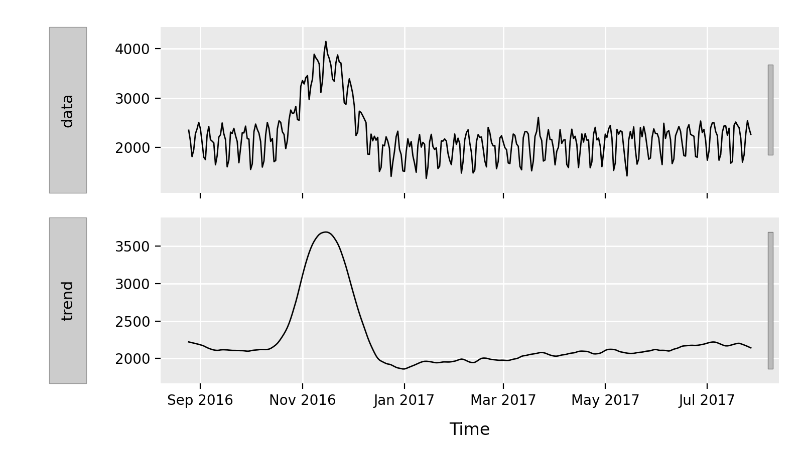
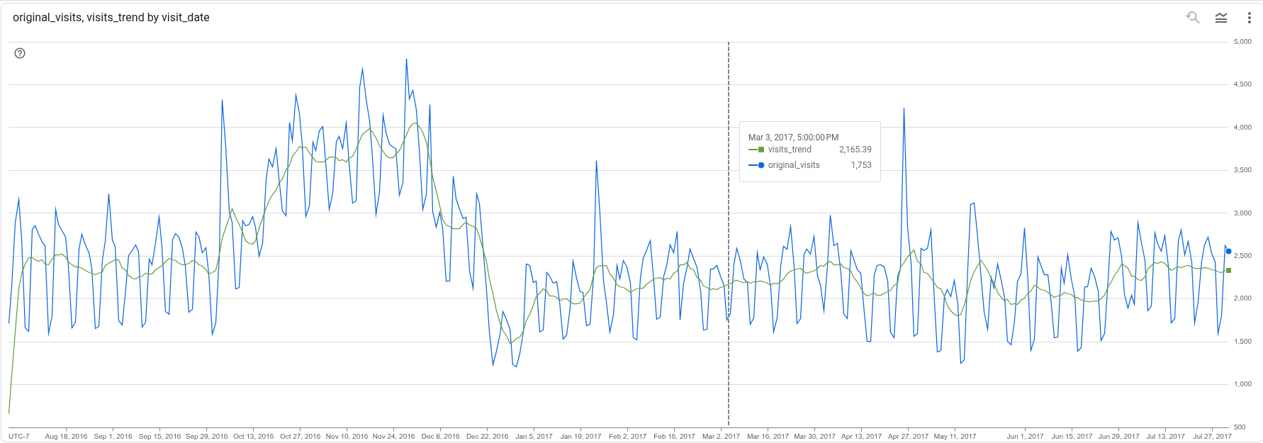
The following example demonstrates how to find the trend component for total website visits over time from publicly available Google Analytics 360 data:
WITH DailyVisits AS (
  SELECT
    PARSE_TIMESTAMP('%Y%m%d', date) AS visit_timestamp,
    SUM(totals.visits) AS total_visits
  FROM
    `bigquery-public-data.google_analytics_sample.ga_sessions_*`
  GROUP BY
    visit_timestamp
)
SELECT
  *
FROM
  ML.TREND(
    TABLE DailyVisits,
    data_col => 'total_visits',
    timestamp_col => 'visit_timestamp'
  )
ORDER BY
  visit_timestamp;
The result is similar to the following:
+-----------------+------------------+--------------+--------------------+
| visit_timestamp | time_series_type | total_visits | trend              |
+-----------------+------------------+--------------+--------------------+
| 2016-08-01      | history          | 1711.0       | 663.58261817132723 |
| 2016-08-02      | history          | 2140.0       | 1108.5377263889254 |
| 2016-08-03      | history          | 2890.0       | 1615.04323567092   |
| ...             | ...              | ...          |                    |
+-----------------+------------------+--------------+--------------------+
What's next
- Learn more about forecasting.
- Learn more about seasonality decomposition.
- Learn more about anomaly detection.