
The ML.SEASONALITY function
This document describes the ML.SEASONALITY function, which lets you
obtain seasonality insights from time series data. The seasonality component
of a time series represents repeating patterns over fixed time periods
in your data, such as years, weeks, or days. For example, your business
might see a small spike in sales every weekend and a larger spike in sales
every year around particular holidays.
The ML.SEASONALITY function is built using the algorithm that is used for the
ARIMA_PLUS model. For more information, see
ARIMA_PLUS: Large-scale, Accurate, Automatic and Interpretable In-Database Time
Series Forecasting and Anomaly Detection in Google BigQuery.
Use the ML.SEASONALITY function to quickly decompose
a time series and view seasonal effects. For a more detailed explanation of the
trend component, see
Seasonal and trend decomposition.
Syntax
ML.SEASONALITY(
  { TABLE TABLE_NAME | (QUERY_STATEMENT) },
  data_col => 'DATA_COL',
  timestamp_col => 'TIMESTAMP_COL'
  [, id_cols => [ID_COLS]]
  [, seasonalities => [SEASONALITIES]]
  [, horizon => HORIZON]
)
Arguments
ML.SEASONALITY takes the following arguments:
TABLE_NAME: the name of the table that contains the time series data to analyze.QUERY_STATEMENT: a GoogleSQL query that produces the time series data to analyze.DATA_COL: aSTRINGvalue that specifies the name of the column that contains the time series data. The data column must use one of the following data types:INT64,NUMERIC,BIGNUMERIC, orFLOAT64.TIMESTAMP_COL: aSTRINGvalue that specifies the name of the column that contains the timestamp data. The timestamp column must use one of the following data types:TIMESTAMP,DATE, orDATETIME.ID_COLS: anARRAY<STRING>value that specifies the names of one or more ID columns. Each unique combination of IDs identifies a unique time series to analyze. Specify one or more values for this argument to analyze multiple time series using a single query. The columns that you specify must use one of the following data types:STRING,INT64,ARRAY<STRING>, orARRAY<INT64>.SEASONALITIES: anARRAY<STRING>value that specifies the seasonality types to extract. Valid values includeYEARLY,QUARTERLY,MONTHLY,WEEKLY, andDAILY. If omitted, the function automatically detects all seasonalities.HORIZON: anINT64value that specifies the number of future time points to forecast for seasonality. The default value is0, which returns results for the historical data only. The valid input range is[1, 10000].
Output
ML.SEASONALITY returns a table with the following columns:
- The columns specified in the
ID_COLSargument. - The input timestamp column.
time_series_type: ASTRINGvalue that indicates whether the row represents historical data (history) or forecasted data (forecast).- The input column specified for
data_colthat contains the data of the time series. For rows wheretime_series_typeishistory, this is either the training data or the interpolated value. For rows wheretime_series_typeisforecast, this is the forecasted value. yearly,quarterly,monthly,weekly,daily:FLOAT64values that contain the calculated seasonal components for each time point. If specific seasonalities are provided in theseasonalitiesargument, only those columns are returned. If no seasonal pattern is detected for a specific component, the value isNULL.status: ASTRINGvalue that contains error messages for invalid input. This column is empty for successful requests.
Example
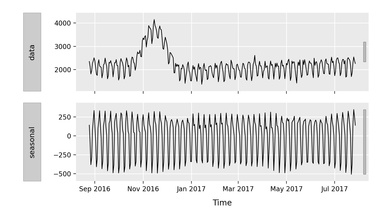
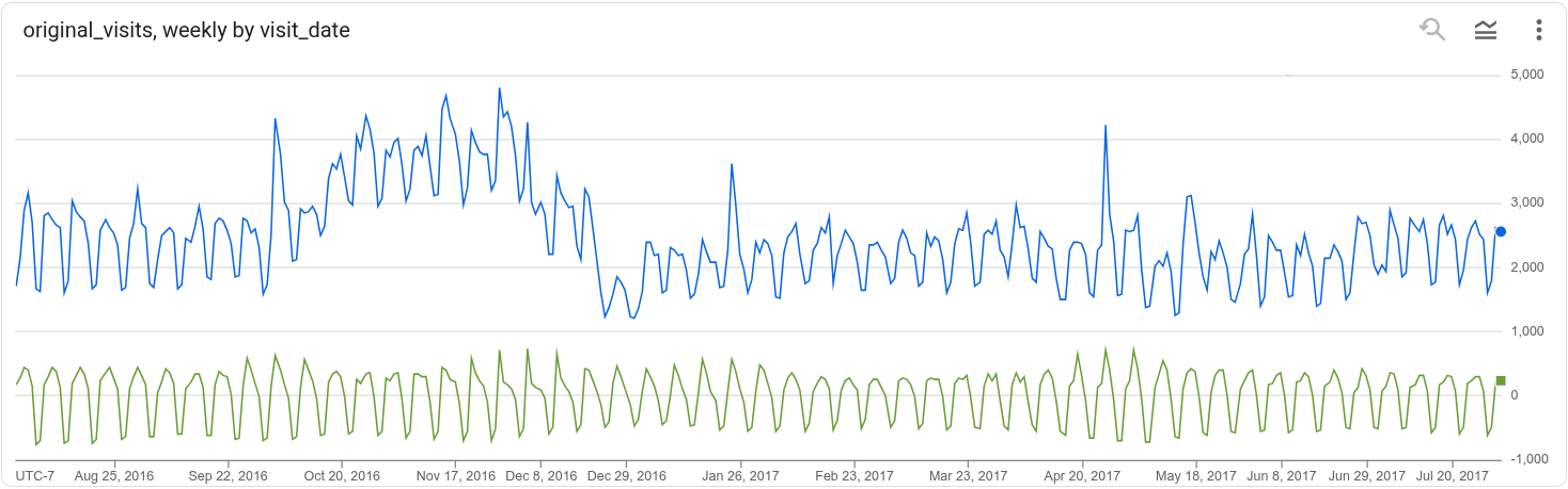
The following example demonstrates how to find the seasonality component for total website visits over time from publicly available Google Analytics 360 data:
WITH DailyVisits AS (
  SELECT
    PARSE_TIMESTAMP('%Y%m%d', date) AS visit_timestamp,
    SUM(totals.visits) AS total_visits
  FROM
    `bigquery-public-data.google_analytics_sample.ga_sessions_*`
  GROUP BY
    visit_timestamp
)
SELECT
  *
FROM
  ML.SEASONALITY(
    TABLE DailyVisits,
    data_col => 'total_visits',
    timestamp_col => 'visit_timestamp'
  )
ORDER BY
  visit_timestamp;
The result is similar to the following:
+------------+------------------+--------------+--------+-----------+---------+--------------------+-------+--------+
| visit_date | time_series_type | total_visits | yearly | quarterly | monthly | weekly             | daily | status |
+------------+------------------+--------------+--------+-----------+---------+--------------------+-------+--------+
| 2016-08-01 | history          | 1711.0       | null   | null      | null    | 169.61193783007687 | null  |        |
| 2016-08-02 | history          | 2140.0       | null   | null      | null    | 287.0332731997334  | null  |        |
| 2016-08-03 | history          | 2890.0       | null   | null      | null    | 445.14087763116709 | null  |        |
| ...        | ...              | ...          | ...    | ...       | ...     | ...                | ...   | ...    |
+------------+------------------+--------------+--------+-----------+---------+--------------------+-------+--------+
The NULL values for the yearly, quarterly, monthly, and daily columns
indicate that no seasonality was detected for those time periods.
What's next
- Learn more about forecasting.
- Learn more about trend decomposition.
- Learn more about anomaly detection.