Work with measures

Note: This feature may not be available when using reservations that are created with certain BigQuery editions. For more information about which features are enabled in each edition, see Introduction to BigQuery editions.

This document shows you how to define and query measures on your graphs. You can use measures to ensure that aggregations are performed correctly across joins.

Overview

A measure is an aggregate property defined within the PROPERTIES clause of a node or edge table. Measures are defined by a measure expression, which is created by using the MEASURE keyword around one of the following:

• an aggregate expression
• an expression that combines aggregate functions with scalar operations
• a derived measure, which is a combinations of measures wrapped in the AGG function that are defined on the same element table

Measures support the following aggregate functions:

• SUM
• AVG
• COUNT
• MIN
• MAX
• AGG (for derived measures)

All aggregate functions except AGG support the DISTINCT keyword. For more information about supported measure expression, read about the measure type.

Measures define their aggregation in reference to the KEY of the node or edge table on which they're defined. This means that when you query a measure, the aggregation is performed correctly even if the underlying table is joined in a way that causes rows to be duplicated.

You can't reference a property defined by a measure in a GQL query. Instead, you access measures by calling the GRAPH_EXPAND TVF to query a relational representation of your graph. By default, GRAPH_EXPAND returns a flattened table representation of your graph with one column per property. You can also specify flatten_results => FALSE to return a hierarchical table with nested STRUCT columns. If your graph contains multiple root node tables, you can specify the start_node argument to choose which root table to traverse.

This function doesn't accept all types of graphs. For more information about which graphs form valid input, see the input limitations. To run GQL queries, you must have a reservation that uses the Enterprise or Enterprise Plus edition. If you use on-demand pricing, you can call the GRAPH_EXPAND function to run SQL queries on your graph.

You can call the AGG function on output from the GRAPH_EXPAND TVF to aggregate the properties according to the aggregation defined in the measure.

Define measures

You define measures within the PROPERTIES clause of a node or edge table definition by using the MEASURE() keyword around a measure expression.

The following example creates a dataset called university and tables for colleges, departments, and courses:

CREATE SCHEMA IF NOT EXISTS university;

CREATE OR REPLACE TABLE university.College (
  college_id INT64 PRIMARY KEY NOT ENFORCED,
  college_name STRING
);

CREATE OR REPLACE TABLE university.Department (
  dept_id INT64 PRIMARY KEY NOT ENFORCED,
  dept_name STRING,
  college_id INT64,
  budget FLOAT64,
  FOREIGN KEY (college_id) REFERENCES university.College(college_id) NOT ENFORCED
);

CREATE OR REPLACE TABLE university.Course (
  course_id INT64 PRIMARY KEY NOT ENFORCED,
  course_name STRING,
  dept_id INT64,
  credits INT64,
  FOREIGN KEY (dept_id) REFERENCES university.Department(dept_id) NOT ENFORCED
);

INSERT INTO university.College (college_id, college_name)
VALUES (101, 'College of Engineering'),
       (102, 'College of Arts');

INSERT INTO university.Department (dept_id, dept_name, college_id, budget)
VALUES (1001, 'Computer Science', 101, 500000),
       (1002, 'Mechanical Engineering', 101, 400000),
       (1003, 'Fine Arts', 102, 200000),
       (1004, 'Research', 101, 50000);

INSERT INTO university.Course (course_id, course_name, dept_id, credits)
VALUES (1, 'Intro to CS', 1001, 3),
       (2, 'Data Structures', 1001, 4),
       (3, 'Thermodynamics', 1002, 3),
       (4, 'Oil Painting', 1003, 2);

The following statement creates a graph called SchoolGraph that defines measures on properties in the Department and Course nodes. You must provide an alias for properties defined by a measure.

CREATE OR REPLACE PROPERTY GRAPH university.SchoolGraph
  NODE TABLES (
    university.College
      KEY(college_id)
      PROPERTIES(college_id, college_name),
    university.Department
      KEY(dept_id)
      PROPERTIES(dept_id, dept_name, college_id,
        budget OPTIONS(description="Department budget in USD"),
        MEASURE(SUM(budget)) AS total_budget,
        MEASURE(SUM(budget) * 1.10) AS budget_with_overhead OPTIONS(
          description="Total department budget including 10% overhead",
          extensions=[("unit", "USD"), ("tier", "planning")]
        )),
    university.Course
      KEY(course_id)
      PROPERTIES(
        course_id,
        course_name,
        credits,
        dept_id,
        MEASURE(AVG(credits)) AS avg_credits,
        MEASURE(SUM(credits)) AS total_credits,
        MEASURE(COUNT(course_id)) AS course_count,
        MEASURE(COUNT(DISTINCT CASE WHEN credits >= 3 THEN course_id ELSE NULL END)) AS major_course_count,
        MEASURE(SAFE_DIVIDE(AGG(total_credits), NULLIF(AGG(course_count), 0))) AS computed_avg_credits)
  )
  EDGE TABLES (
    university.Department AS CollegeDept
      SOURCE KEY (college_id) REFERENCES College (college_id)
      DESTINATION KEY (dept_id) REFERENCES Department (dept_id),
    university.Course AS DeptCourse
      SOURCE KEY (dept_id) REFERENCES Department (dept_id)
      DESTINATION KEY (course_id) REFERENCES Course (course_id)
  );

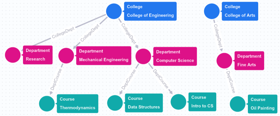
The total_budget measure is defined as MEASURE(SUM(budget)). The measure locks the aggregation to the KEY, which is dept_id.

Derived measures

A derived measure is a measure that references other measures defined on the same element table by using the AGG() function. This functionality lets you build reusable measure hierarchies.

For example, in university.Course, the computed_avg_credits measure calculates the ratio between the measures total_credits and course_count:

MEASURE(SAFE_DIVIDE(AGG(total_credits), NULLIF(AGG(course_count), 0))) AS computed_avg_credits

Derived measures retain the grain-locking property of the underlying element table key. Measure dependencies are resolved at graph compilation time. Circular references between measures return an error.

Understanding overcounting

When you join tables, data is repeated every time there is a one-to-many relationship in your data. For example, if you join the Course, Department, and College tables, a department with multiple courses appears in multiple rows in the output:

SELECT
  college_name,
  dept_name,
  course_name,
  budget
FROM university.Course
LEFT JOIN university.Department
  ON Course.dept_id = Department.dept_id
LEFT JOIN university.College
  ON Department.college_id = College.college_id;

/*------------------------+------------------------+-----------------+----------+
 | college_name           | dept_name              | course_name     | budget   |
 +------------------------+------------------------+-----------------+----------+
 | College of Engineering | Computer Science       | Intro to CS     | 500000.0 |
 | College of Engineering | Computer Science       | Data Structures | 500000.0 |
 | College of Engineering | Mechanical Engineering | Thermodynamics  | 400000.0 |
 | College of Arts        | Fine Arts              | Oil Painting    | 200000.0 |
 +------------------------+------------------------+-----------------+----------*/

If you try to compute the total budget per college using SUM(budget), the Computer Science department's budget is counted twice. You can avoid this problem by querying the Department table directly, but this approach doesn't work if you want to compute multiple aggregations from different tables that contribute to your joined data. The following section shows how measures solve this problem.

Query a graph with measures

You can query a graph with measures using GQL, but your query can't directly reference any property defined by a measure. For example, the following query references nodes that have measure properties defined, but doesn't use or return any of the measure fields:

GRAPH university.SchoolGraph
MATCH (c:College)->(d:Department)->(course:Course)
RETURN c.college_name, d.dept_name, course.course_name;

/*------------------------+------------------------+-----------------+
 | college_name           | dept_name              | course_name     |
 +------------------------+------------------------+-----------------+
 | College of Engineering | Computer Science       | Intro to CS     |
 | College of Engineering | Computer Science       | Data Structures |
 | College of Engineering | Mechanical Engineering | Thermodynamics  |
 | College of Arts        | Fine Arts              | Oil Painting    |
 +------------------------+------------------------+-----------------*/

To work with measures, you use the GRAPH_EXPAND table-valued function (TVF) to query your graph as a relational table:

GRAPH_EXPAND(
  graph_name [, start_node => 'NodeName'] [, flatten_results => TRUE|FALSE]
)

The function accepts the following arguments:

• graph_name: A STRING containing the name of the graph.
• start_node: An optional STRING specifying the starting node table for traversal. This argument is required if the graph has multiple root node tables.
• flatten_results: An optional BOOL (defaults to TRUE):
  • TRUE: Flattens all node and edge properties into top-level columns with <element>_<property> prefixes.
  • FALSE: Returns the root node properties as un-prefixed top-level columns and joined neighbor tables as STRUCT columns.

Use flattened output

When flatten_results is set to TRUE (the default mode), columns in the output table are named by concatenating the node or edge table label and the property name—for example, Course_course_name or Department_total_budget. The following query shows sample output from the GRAPH_EXPAND TVF:

SELECT
  College_college_name,
  Department_dept_name,
  Department_budget,
  Course_course_name
FROM
  GRAPH_EXPAND("university.SchoolGraph");

/*------------------------+------------------------+-------------------+--------------------+
 | College_college_name   | Department_dept_name   | Department_budget | Course_course_name |
 +------------------------+------------------------+-------------------+--------------------+
 | College of Engineering | Computer Science       | 500000.0          | Intro to CS        |
 | College of Engineering | Computer Science       | 500000.0          | Data Structures    |
 | College of Engineering | Mechanical Engineering | 400000.0          | Thermodynamics     |
 | College of Arts        | Fine Arts              | 200000.0          | Oil Painting       |
 +------------------------+------------------------+-------------------+--------------------*/

The GRAPH_EXPAND function produces the flattened table by applying a series of LEFT JOIN operations to node and edge tables. If you don't specify a starting node, then the input graph must have a single root node table in the schema relationship graph. Equivalently, the root node table must have a many-to-one relationship with every other node table that it shares an edge with. Data that isn't reachable from the root node table through a series of joins doesn't appear in the output. In the previous example, Course is the root node table. The Research department is omitted from the output because it doesn't have any courses.

You can't directly select a column for a property defined by a measure. Instead, you must wrap them in the AGG() function. This function ensures that the aggregation defined on the measures is performed exactly once per key.

The following query simultaneously calculates the total budget and total number of courses for each college:

SELECT
  College_college_name,
  AGG(Department_total_budget) AS college_budget,
  AGG(Course_course_count) AS total_courses
FROM
  GRAPH_EXPAND("university.SchoolGraph")
GROUP BY
  College_college_name;

/*------------------------+----------------+---------------+
 | College_college_name   | college_budget | total_courses |
 +------------------------+----------------+---------------+
 | College of Engineering | 900000.0       | 3             |
 | College of Arts        | 200000.0       | 1             |
 +------------------------+----------------+---------------*/

Use hierarchical output

When you specify flatten_results => FALSE, GRAPH_EXPAND returns a hierarchical relation instead of prefixed columns:

• Properties of the starting root node appear as un-prefixed top-level columns (for example, course_name or credits).
• Properties of joined neighbor tables, which might be node or edge tables, appear as nested STRUCT fields named after the element table. For example, if the starting node is Course, then you would use DeptCourse.Department.CollegeDept.College.college_nameto access thecollege_name` property.
• Measures inside nested structs are queried using dot notation inside AGG()—for example, AGG(DeptCourse.Department.total_budget).
• If an element table has a property with the same name as an adjacent element table, then you can't query the graph using flatten_results => FALSE. You must flatten the results instead.

SELECT
  DeptCourse.Department.dept_name AS department_name,
  DeptCourse.Department.CollegeDept.College.college_name,
  AGG(DeptCourse.Department.total_budget) AS total_budget,
  AGG(course_count) AS total_courses
FROM GRAPH_EXPAND(
       "university.SchoolGraph",
       start_node => "Course",
       flatten_results => FALSE)
GROUP BY department_name, college_name;

Work with multiple root node tables

Graphs often contain multiple root node tables, also called fact tables, that share dimension tables. To query a graph with multiple root node tables, use the start_node argument in GRAPH_EXPAND. The function traverses the subgraph reachable from the starting node.

For example, you can add an Instructor table to the university dataset that also links to Department:

CREATE OR REPLACE TABLE university.Instructor (
  instructor_id INT64 PRIMARY KEY NOT ENFORCED,
  instructor_name STRING,
  dept_id INT64,
  salary FLOAT64,
  FOREIGN KEY (dept_id) REFERENCES university.Department(dept_id) NOT ENFORCED
);

INSERT INTO university.Instructor (instructor_id, instructor_name, dept_id, salary)
VALUES (501, 'Dr. Dana', 1001, 120000),
       (502, 'Dr. Lee', 1001, 110000),
       (503, 'Dr. Taylor', 1002, 115000),
       (504, 'Prof. Izumi', 1003, 90000);

You can create a new graph called university.SchoolGraphMultiRoot that includes the Instructor node table and an edge from Instructor to Department:

CREATE OR REPLACE PROPERTY GRAPH university.SchoolGraphMultiRoot
  NODE TABLES (
    university.College
      KEY(college_id)
      PROPERTIES(college_id, college_name),
    university.Department
      KEY(dept_id)
      PROPERTIES(dept_id, dept_name, college_id, budget,
        MEASURE(SUM(budget)) AS total_budget),
    university.Course
      KEY(course_id)
      PROPERTIES(
        course_id, course_name, credits, dept_id,
        MEASURE(COUNT(course_id)) AS course_count),
    university.Instructor
      KEY(instructor_id)
      PROPERTIES(
        instructor_id, instructor_name, dept_id, salary,
        MEASURE(COUNT(instructor_id)) AS instructor_count,
        MEASURE(SUM(salary)) AS total_salary)
  )
  EDGE TABLES (
    university.Department AS CollegeDept
      SOURCE KEY (college_id) REFERENCES College (college_id)
      DESTINATION KEY (dept_id) REFERENCES Department (dept_id),
    university.Course AS DeptCourse
      SOURCE KEY (dept_id) REFERENCES Department (dept_id)
      DESTINATION KEY (course_id) REFERENCES Course (course_id),
    university.Instructor AS DeptInstructor
      SOURCE KEY (dept_id) REFERENCES Department (dept_id)
      DESTINATION KEY (instructor_id) REFERENCES Instructor (instructor_id)
  );

In this graph, both Course and Instructor serve as root node tables that link to Department and College. You can target either subgraph by passing start_node:

-- Expand the Course subgraph (Course -> Department -> College)
SELECT
  College_college_name,
  AGG(Course_course_count) AS total_courses
FROM GRAPH_EXPAND("university.SchoolGraphMultiRoot", start_node => "Course")
GROUP BY College_college_name;

-- Expand the Instructor subgraph (Instructor -> Department -> College)
SELECT
  College_college_name,
  AGG(Instructor_total_salary) AS total_faculty_salary
FROM GRAPH_EXPAND("university.SchoolGraphMultiRoot", start_node => "Instructor")
GROUP BY College_college_name;

To analyze metrics across multiple fact tables, query each subgraph by using GRAPH_EXPAND and join them on their shared dimensions in standard SQL:

SELECT
  C.College_college_name,
  AGG(C.Course_course_count) AS total_courses,
  AGG(I.Instructor_total_salary) AS total_faculty_salary
FROM GRAPH_EXPAND("university.SchoolGraphMultiRoot", start_node => "Course") AS C
INNER JOIN GRAPH_EXPAND("university.SchoolGraphMultiRoot", start_node => "Instructor") AS I
  ON C.Department_dept_id = I.Department_dept_id
GROUP BY C.College_college_name;

Both AGG(C.Course_course_count) and AGG(I.Instructor_total_salary) calculate their aggregations accurately at their respective grains without interference from the join.

Caution: Changes to the underlying graph don't invalidate cached results for queries that call the GRAPH_EXPAND function. To ensure correct output, disable the retrieval of cached results when you call this function.

Best practices

When you design a graph with measures, follow these best practices:

Define nodes and edges within a single table

We recommend that you use the same table for a node table definition and its connecting edge table definitions. Reusing the table ensures a one-to-one (1:1) relationship between the node table and the edge table, which prevents fan-out and ensures that the GRAPH_EXPAND function doesn't ignore the edge as ambiguous.

For example, if you have an input table Enrollment that contains foreign keys pointing to Student and Course tables, define the Enrollment node and its outgoing edges using the Enrollment input table.

Avoid defining unnecessary properties on edge tables

When you define a node table and an edge table using the same physical table, don't use the PROPERTIES clause on the edge table unless there's new information to capture on the edge. Because the node table and edge table use the same physical table, all of these properties are already part of the node table.

Defining redundant properties on the edge table can cause the GRAPH_EXPAND function to treat the edge table as a separate entity from the shared node table. To optimize performance, specify NO PROPERTIES on the edge table definition when there are no new properties to capture on the edge.

Model many-to-many relationships as node tables

A many-to-many (M:N) relationship occurs when a row in table A can correspond to multiple rows in table B, and a row in table B can correspond to multiple rows in table A. For example, one student can enroll in multiple courses and one course can have many students. You can separate a many-to-many relationship into two one-to-many relationships by using an intermediate junction table. For example, you can define an Enrollment table that contains foreign keys pointing to Student and Course tables. If you model an intermediate junction table as an edge table that connects two dimension node tables in your CREATE PROPERTY GRAPH statement, such as in the following example, then the GRAPH_EXPAND function ignores these edges because their relationship is ambiguous: not clearly many-to-one or one-to-one.

CREATE PROPERTY GRAPH university.SchoolGraph
  NODE TABLES (
    university.Student,
    university.Course
  )
  EDGE TABLES (
    -- Modeling the junction table as a standalone edge causes ambiguity
    university.Enrollment AS StudentEnrollment
      SOURCE KEY (student_id) REFERENCES Student (student_id)
      DESTINATION KEY (course_id) REFERENCES Course (course_id)
  );

If all edges in a graph are ignored, calls to GRAPH_EXPAND or BQ.SHOW_GRAPH_EXPAND_SCHEMA fail with an error.

To correctly model an M:N relationship for measures, promote the intermediate junction table to a node table. In this structure, the junction node table serves as the single root node table (a node table with an in-degree of zero). Then, define two many-to-one (N:1) edge tables that share the junction table to connect N:1 to each of the dimension node tables:

CREATE PROPERTY GRAPH university.SchoolGraph
  NODE TABLES (
    university.Student KEY (student_id),
    university.Course KEY (course_id),
    -- Promote the junction table to a node table (acting as the single root node)
    university.Enrollment KEY (enrollment_id)
  )
  EDGE TABLES (
    -- Share (reuse) the Enrollment table to define N:1 edges to each dimension
    university.Enrollment AS EnrollmentToStudent
      SOURCE KEY (enrollment_id) REFERENCES Enrollment (enrollment_id)
      DESTINATION KEY (student_id) REFERENCES Student (student_id),
    university.Enrollment AS EnrollmentToCourse
      SOURCE KEY (enrollment_id) REFERENCES Enrollment (enrollment_id)
      DESTINATION KEY (course_id) REFERENCES Course (course_id)
  );

In this structure, Enrollment serves as the single root node table (in-degree of zero) connecting N:1 to the Student and Course dimension tables (in-degree of one). The GRAPH_EXPAND function can flatten this graph by traversing outwards from Enrollment to Student and Course. If you define measures on any of these tables, you can call the AGG function on the measure columns to correctly compute the aggregations without overcounting.

Choose how measures handle unmatched rows

When a row has no match in a connected element table, the columns of that table are NULL in the GRAPH_EXPAND output. For example, if a course has no dept_id value, then the Department columns of that row are NULL. Whether a measure on the Department node includes these rows depends on where you write the scalar expression that the measure aggregates.

If you write the expression inside the aggregate function, then the expression is evaluated for every row of the expanded output, including rows with no match. When the expression returns a value rather than NULL for one of these rows, that value contributes to the result.

If you define the expression as a property and reference that property from the measure, then the expression is evaluated on the rows of the node table, and rows with no match don't contribute to the result.

The following example defines the same expression both ways on university.Department:

university.Department
  KEY(dept_id)
  PROPERTIES(dept_id, dept_name, college_id, budget,
    COALESCE(budget, 0) AS budget_or_zero,
    -- Includes courses that have no department, as a budget of 0.
    MEASURE(AVG(COALESCE(budget, 0))) AS avg_budget_inline,
    -- Averages only departments that exist.
    MEASURE(AVG(budget_or_zero)) AS avg_budget_property)

Both measures replace a NULL budget with 0. The inline form also replaces the NULL values produced for a course that has no department, so that course is averaged in as a department with a budget of 0. Choose the form that matches what you want to measure.

View GRAPH_EXPAND schema

To view the schema of the table returned by the GRAPH_EXPAND function without calling the function, use the BQ.SHOW_GRAPH_EXPAND_SCHEMA system procedure:

DECLARE schema STRING DEFAULT '';
CALL BQ.SHOW_GRAPH_EXPAND_SCHEMA('university.SchoolGraph', schema);
SELECT schema;

This procedure populates the schema variable with the name, type, and mode of each column. It also indicates whether the property referenced by the column is a measure, and lists any description or synonyms that you defined on it.

What's next

• Learn how to create and query a graph.
• Learn about graph schemas.