

Given a directed graph with non-negative edge weights, this algorithm computes a shortest path between every node in a supplied source nodes set \(S\) and every node in a supplied target nodes set \(T\). For each \(s \in S, t \in T\), the algorithm finds a path from \(s\) to \(t\) that minimizes the shortest-path distance, defined as the sum of the weights of the path's edges. If multiple shortest paths exist between \(s\) and \(t\) (all with the same distance), the algorithm chooses one of the paths in a deterministic way: first, it selects path(s) containing a minimal number of edges, and if there are multiple such paths, it breaks ties by picking the path that minimizes the node IDs along the reverse paths from \(t\) back to \(s\) (see this example).
Interface specifications
The following list summarizes the expectations on the graph passed as input to this algorithm. These expectations complement the ones listed in General assumptions on input graphs.
- Directed graph (an undirected graph can be converted into a directed graph by replacing each undirected edge \(xy\) with two directed edges \(xy\) and \(yx\), both with the same weight as the original edge).
- Edge weights: Must be non-negative.
Self-loops are always ignored because they will never be part of any shortest path.
The algorithm also takes as input a list of source node IDs and target node IDs defining the source and target node sets \(S\) and \(T\). Both of these lists must be nonempty and contain valid node IDs, that is, IDs between 0 (inclusive) and the number of nodes in the graph (exclusive). The same node ID may appear in both lists (in which case the shortest path between a node and itself will be the empty path with distance 0.0).
The result contains a total of \(|S| \times |T|\) shortest path distances and the sequence of intermediate nodes along each shortest path (to avoid including the IDs of \(s\) and \(t\) themselves in the path result). If no path exists between a given source and target, the algorithm returns a distance of -1.0, and the corresponding intermediate node list will be empty.
To obtain only the shortest-path distances, use this configuration parameter to suppress the computation and returning of the intermediate nodes along each path:
| Name | Type | Description |
|---|---|---|
return_paths
|
bool | If true, return for each source \(s\) and target
\(t\) the intermediate nodes of the shortest path
from \(s\) to \(t\). |
Algorithm
The algorithm reduces the many-to-many shortest paths computation to multiple single-source shortest path (SSSP) computations: for each source node \(s \in S\) (one at a time), the algorithm runs a parallel SSSP algorithm from \(s\) to obtain the shortest-path tree rooted at \(s\).
The SSSP algorithm is an implementation of the \(\rho\)-stepping algorithm from Efficient Stepping Algorithms and Implementations for Parallel Shortest Paths (Symposium on Parallelism in Algorithms and Architectures, 2021). \(\rho\)-stepping belongs to a family of stepping algorithms for parallel SSSP. These algorithms maintain a priority queue of active nodes (nodes whose distance estimates have improved but whose outgoing edges have not yet been relaxed, that is, used to update the distance estimates of their neighbors) and proceed in synchronous rounds. In each round, the algorithm extracts a set of nodes from the queue based on a distance threshold, and relaxes their outgoing edges in parallel.
The key idea of \(\rho\)-stepping is to choose the extraction threshold adaptively based on the size of the frontier. If the frontier contains fewer than \(\rho\) nodes, the algorithm sets the threshold so that it processes all frontier nodes. Otherwise, the algorithm uses a sampling scheme to estimate a threshold such that it will extract approximately \(\rho\) nodes: it randomly samples a subset of the frontier, sorts the samples by distance, and picks the threshold from an appropriate rank in the sorted order.
Computational complexity
The algorithm is a parallel algorithm. For a single SSSP computation, it runs in \(O(D \cdot m \cdot \log(n^2 / (m \rho)))\) work and \(O(D \cdot n \cdot \log(n) / \rho)\) depth, where \(n\) and \(m\) denote the number of nodes and edges in the input graph, respectively, and \(D\) is the depth of the shortest-path tree (the maximum number of hops in any shortest path from the source). Running the algorithm on a machine that supports high amounts of parallelism tends to lead to a smaller running time.
Since the many-to-many algorithm runs one SSSP per source node sequentially, the overall work and depth are each multiplied by \(|S|\).
The memory used by the algorithm is \(O(n + |S| \cdot |T|)\) when return_paths
is false, or \(O(n + |S| \cdot |T| \cdot D)\) when return_paths is true.
Example
Consider this directed graph consisting of 11 nodes labeled \(a\) to \(k\) (representing the integer node IDs 0 through 10 in order):
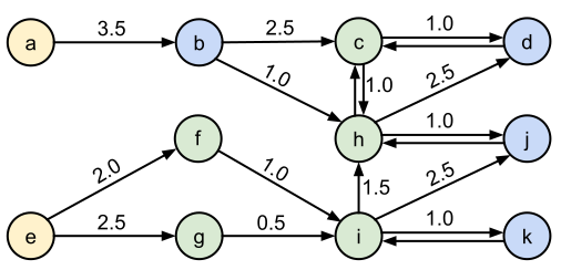
Running the algorithm with \(S = \{a, e\}\) (yellow nodes) and \(T = \{b, d, j, k\}\) (blue nodes) yields these results:
- \(a \rightarrow b\): distance = 3.5, intermediate nodes = \([]\)
- \(a \rightarrow d\): distance = 6.5, intermediate nodes = \([b, h, c]\)
- \(a \rightarrow j\): distance = 5.5, intermediate nodes = \([b, h]\)
- \(a \rightarrow k\): distance = -1.0, intermediate nodes = \([]\)
- \(e \rightarrow b\): distance = -1.0, intermediate nodes = \([]\)
- \(e \rightarrow d\): distance = 6.5, intermediate nodes = \([f, i, h, c]\)
- \(e \rightarrow j\): distance = 5.5, intermediate nodes = \([f, i]\)
- \(e \rightarrow k\): distance = 4.0, intermediate nodes = \([f, i]\)
Note that:
- Because there is a direct edge from node \(a\) to node \(b\), the list of intermediate nodes in the shortest path is empty.
- Because there is no path from node \(a\) to node \(k\) (or from node \(e\) to node \(b\)), the distance is -1.0, and the list of intermediate nodes is empty.
- Path distances are defined by the sum of the edge weights along the path, not by the number of edges in the path (although the latter is part of the tie-breaking algorithm, as described next). For example, in determining the shortest path from node \(a\) to node \(d\), the algorithm selects the path \([a, b, h, c, d]\) of distance 6.5 over the path \([a, b, c, d]\) with distance 7.0 even though the latter path is composed of fewer edges.
- If there are multiple shortest paths, the algorithm chooses one deterministically. For example, there are actually 4 shortest paths in the graph from node \(e\) to node \(j\), all with length 5.5: \([e, f, i, j]\), \([e, f, i, h, j]\), \([e, g, i, j]\), and \([e, g, i, h, j]\). In determining which path to return, the algorithm considers only those paths involving the minimal number of edges. That rules out the 4-edge paths \([e, f, i, h, j]\) and \([e, g, i, h, j]\), leaving the 3-edge paths \([e, f, i, j]\) and \([e, g, i, j]\). Among these remaining paths, the algorithm breaks ties as follows. In theory, it considers the paths starting at the target node and working backwards toward the source, comparing node IDs at the same relative position within the paths. At the first difference, it chooses the path with the smaller node ID. In this case, the last and second-to-last node IDs are the same. The first difference is at the second position. Note that \(f\) and \(g\) denote nodes 5 and 6; since \(5 < 6\), the algorithm selects the path \([e, f, i, j]\). In practice, the algorithm does this efficiently without having to consider all fewest-edges shortest paths.
- This example does not illustrate that in the degenerate case that the same node ID appears in both \(S\) and \(T\), the shortest path distance from the node to itself will be 0.0, and the list of intermediate nodes will be empty.
External references
- The \(\rho\)-stepping algorithm was introduced in Efficient Stepping Algorithms and Implementations for Parallel Shortest Paths (Symposium on Parallelism in Algorithms and Architectures, 2021).