

This algorithm computes pairwise node similarities for given sets of source nodes and target nodes of a directed graph with edge weights that may be negative, zero, or positive. The algorithm supports multiple similarity metrics, all of which are symmetric—that is, for two nodes \(x\) and \(y\), the similarity between \(x\) and \(y\) is equal to the similarity between \(y\) and \(x\).
Similarity metrics
Let \(N(x)\) denote the set of out-neighbors of a node \(x\), and let \(w_{xy}\) denote the weight of an edge \(xy\). The similarity metrics for a pair of nodes \(x\) and \(y\) are defined as follows.
Common neighbors similarity
The similarity is defined as the number of neighbors that \(x\) and \(y\) have in common:
\[CN(x, y) = |N(x) \cap N(y)|.\]
This similarity measure ignores edge weights.
Total neighbors similarity
The similarity is defined as the number of unique nodes in the union of the out-neighbor sets of \(x\) and \(y\):
\[TN(x, y) = |N(x) \cup N(y)|.\]
This similarity measure ignores edge weights.
Jaccard similarity
The similarity is defined as the size of the intersection of their out-neighbor sets divided by the size of the union:
\[ J(x, y) = \frac{CN(x, y)}{TN(x, y)} = \frac{|N(x) \cap N(y)|}{|N(x) \cup N(y)|}. \]
If both out-neighbor sets are empty (that is, \(TN(x, y) = 0\)), the similarity is undefined and the algorithm returns NaN. This similarity measure ignores edge weights.
Cosine similarity
The similarity is defined as:
\[ C(x, y) = \frac{\sum_{z \in N(x) \cap N(y)} w_{xz} w_{yz}} {\sqrt{\sum_{z \in N(x)} w_{xz}^2} \sqrt{\sum_{z \in N(y)} w_{yz}^2}} . \]
If \(x\) or \(y\) has no out-neighbors or either's outgoing edges all have weight 0, then the similarity is undefined and the algorithm returns NaN.
Note that one can equivalently define the cosine similarity in terms of vector operations, as follows. The set of out-neighbors of \(x\) can be viewed as a vector indexed by the nodes of the graph, where the \(z\)-th component is \(w_{xz}\) if \(z \in N(x)\) and 0 otherwise; define a vector for \(y\) in the same manner. The cosine similarity between \(x\) and \(y\) is the cosine of the angle between the vectors of \(x\) and \(y\), which can be computed as the dot product of the vectors divided by the product of their L2 norms.
Interface specifications
The following list summarizes the expectations on the graph passed as input to this algorithm. These expectations complement the ones listed in General assumptions on input graphs.
- Directed graph (an undirected graph can be converted into a directed graph by replacing each undirected edge \(xy\) with two directed edges \(xy\) and \(yx\), both with the same weight as the original edge).
- Edge weights: May be negative, zero, or positive. Used only by cosine similarity; ignored by the other metrics.
In addition to the input graph, the algorithm requires two lists of nonempty
node IDs source_nodes and target_nodes.
The output is a matrix of floating-point numbers, where entry [i][j] contains
the similarity between the nodes source_nodes[i] and target_nodes[j] (or
NaN, if the similarity is undefined).
The following parameter configures the algorithm:
| Name | Type | Description |
|---|---|---|
metric
|
enum | The similarity metric to use. Must be one of JACCARD,
COSINE, COMMON, or TOTAL. |
Computational complexity
Let:
- \(n\) and \(m\) denote the numbers of nodes and edges in the input graph.
- \(S\) and \(T\) denote the sets of source nodes and target nodes respectively.
- \(\Delta\) be the maximum degree of a node in \(S\) or \(T\).
The algorithm is a parallel algorithm that runs in \(O(|S||T|\Delta)\) work and \(O(\Delta)\) depth. Running the algorithm on a machine that supports high amounts of parallelism tends to lead to a smaller running time.
The memory used by the algorithm is \(O(|S||T| + \text{num_threads}\cdot \Delta)\), where \(\text{num_threads}\) is the number of threads used during the algorithm execution.
Example
Consider the following graph with 8 nodes and the given weighted edges:
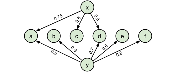
In this example \(N(x) = \{a, c, d\}\) and \(N(y) = \{a, b, d, e, f\}\). Hence, we compute the different similarity metrics as follows:
Common neighbors similarity
\[ CN(x, y) = |N(x) \cap N(y)| = |\{a, c, d\} \cap \{a, b, d, e, f\}| = |\{a, d\}| = 2. \]
Total neighbors similarity
\[ TN(x, y) = |N(x) \cup N(y)| = |\{a, c, d\} \cup \{a, b, d, e, f\}| = |\{a, b, c, d, e, f\}| = 6. \]
Jaccard similarity
\[ J(x, y) = CN(x, y) / TN(x, y) = 2 / 6 = 1/3. \]
Cosine similarity
In this case, the algorithm takes edge weights into account. Using \(N(x) \cap N(y) = \{a, d\}\):
\[ C(x, y) = \frac{(0.75 \cdot 0.5) + (0.8 \cdot 0.7)} {\sqrt{(0.75^2 + 0.6^2 + 0.8^2)} \sqrt{(0.5^2 + 0.9^2 + 0.7^2 + 0.6^2 + 0.8^2)}} = \frac{0.935}{1.25 \cdot 1.59687} = 0.46842. \]
As mentioned in the earlier description of cosine similarity, this similarity metric can also be expressed as the cosine of the angle between the two out-edge sets thought of as vectors. We can convert to a vector representation by assigning the indices \(0, 1, ..., 7\) for the nodes \(a, b, ..., f, x, y\) and using the edge weights for the magnitudes at each position:
\[ \vec{x} = (0.75, 0.0, 0.6, 0.8, 0.0, 0.0, 0.0, 0.0) \\\\ \vec{y} = (0.5, 0.9, 0.0, 0.7, 0.6, 0.8, 0.0, 0.0) \]
The cosine of the angle between these two vectors can be computed by normalizing the two vectors to have unit length and computing their dot product:
\[ \begin{align*} C(x, y) &= \frac{\vec{x}}{||\vec{x}||} \cdot \frac{\vec{y}}{||\vec{y}||} \\\\ &= \frac{(0.75, 0, 0.6, 0.8, 0, 0, 0, 0)}{1.25} \cdot \frac{(0.5, 0.9, 0, 0.7, 0.6, 0.8, 0, 0)}{1.59687} \\\\ &= (0.6, 0, 0.48, 0.64, 0, 0, 0, 0) \cdot (0.31311, 0.56360, 0, 0.43836, 0.37574, 0.50098, 0, 0) \\\\ &= 0.18787 + 0 + 0 + 0.28055 + 0 + 0 + 0 + 0 \\\\ &= 0.46842. \end{align*} \]