

This algorithm computes the closeness centralities of all nodes of a graph with non-negative edge weights. There are multiple (non-equivalent) ways of defining closeness centralities. This page considers two definitions. Depending on which algorithm is chosen (EXACT or HYBRID), the input graph is a directed graph
or an
undirected graph. The following definition of closeness centrality focuses on the case of a directed graph. For the purpose of this definition, one can treat
an undirected graph as a directed graph, by replacing each undirected edge
\(xy\) with two directed edges \(xy\) and \(yx\), both with the same weight as
the original edge. Let:
- \(n\) be the number of nodes in the graph;
- \(d(x, y)\) be the shortest-path distance between nodes \(x\) and \(y\) in the graph, which is defined if and only if there exists a path from \(x\) to \(y\); and
- \(R(x)\) be the set of all nodes \(y\) other than \(x\) such that there exists a path from \(x\) to \(y\).
The (standard) closeness centrality of a node \(x\) is defined as
\[ \text{closeness_centrality}(x) = \ \frac{|R(x)|}{\sum_{y \in R(x)} d(x, y)} . \]
Multiplying the standard closeness centrality of a node \(x\) by \(\frac{|R(x)|}{n - 1}\) yields its Wasserman-Faust closeness centrality:
\[ \text{closeness_centrality}_{WF}(x) = \frac{|R(x)|} {n - 1} \text{closeness_centrality}(x). \]
Note that in the case where the graph is strongly connected, \(|R(x)| = n - 1\) for all nodes \(x\), and the two centrality measures \(\text{closeness_centrality}(x)\) and \(\text{closeness_centrality}_{WF}(x)\) become equivalent.
The cases where the denominator (in either preceding definition) is zero are handled in a special manner. There are two such cases:
- Case 1: \(R(x)\) is empty (note that this also encompasses the case where \(n = 1\)). In this case, the (standard and Wasserman-Faust) closeness centralities of \(x\) are defined as zero.
- Case 2: \(R(x)\) is nonempty, but \(d(x, y) = 0\) for every node \(y \in R(x)\). In this case, the (standard and Wasserman-Faust) closeness centralities of \(x\) are defined as infinity.
Other definitions of closeness centrality
There are other (non-equivalent) definitions of closeness centrality beyond the two definitions that this page uses. See for example the Wikipedia article on closeness centrality for other definitions.
Interface specifications
The following list summarizes the expectations on the graph passed as input to this algorithm. These expectations complement the ones listed in General assumptions on input graphs.
- Directed graph (
EXACTalgorithm) or undirected graph (HYBRIDalgorithm). An undirected graph can be converted into a directed graph by replacing each undirected edge \(xy\) with two directed edges \(xy\) and \(yx\), both with the same weight as the original edge.- Edge weights: Must be non-negative.
The output is a list of \(n\) floating-point numbers, corresponding to the centralities of all nodes. The algorithm may return the standard or Wasserman-Faust closeness centralities, depending on the parameter values.
The following parameters configure the algorithm:
| Name | Type | Description |
|---|---|---|
algorithm
|
enum | Specifies the algorithm to
use. Possible values are
EXACT and HYBRID. |
use_wasserman_faust
|
boolean | Specifies whether the algorithm should compute standard closeness centralities (false) or Wasserman-Faust closeness centralities (true). |
sample_size
|
integer (optional) | Used only by the HYBRID
algorithm. The number of
pivot nodes to use for
approximately computing the
centrality values. Must be
non-negative. If not set or
zero, the algorithm uses
the value
\(\min(100 \ln n, n)\). If
it is set to a value larger
than \(n\), the algorithm
caps the value to \(n\). |
sampling_seed
|
integer (optional) | Used only by the HYBRID
algorithm. The seed for the
random number generator used
for selecting the pivot
nodes. The algorithm selects
the same set of pivot nodes
if given the same input
graph, sample_size, and
sampling_seed. |
epsilon
|
floating-point number (optional) | Used only by the HYBRID
algorithm. Must be in the
range (0.0, 1.0), and
controls how the
centralities are estimated.
See the explanation of the
HYBRID algorithm in the
following section. |
Algorithms
The algorithm provides two modes: EXACT and HYBRID. As the name suggests,
the EXACT algorithm computes the centralities exactly. The HYBRID algorithm,
on the other hand, computes approximate centralities, and is much faster than
the EXACT algorithm for large graphs.
The EXACT algorithm
This algorithm takes a directed graph as input. It runs Dijkstra's single-source shortest-path algorithm \(n\) times (in parallel)—one time with each of the nodes as the source—and uses the shortest-path distances returned by Dijkstra's algorithm to compute the centralities exactly.
The HYBRID algorithm
This algorithm takes an undirected graph as input. It is a randomized
approximation algorithm that samples a small set of sample_size "pivot" nodes
uniformly at random, and then runs Dijkstra's algorithm from each pivot node to
compute the shortest-path distances from the pivots to all other nodes in the
graph. It then uses those distances to estimate the centralities of all the
nodes, as explained in the paragraphs that follow.
The centrality of each pivot node is computed exactly. For a non-pivot node \(x\), the algorithm first checks if there is any pivot node in the same connected component as \(x\). If there is no such pivot node, the algorithm estimates the centrality of \(x\) to be zero. Otherwise, it finds the pivot node \(p(x)\) that is closest to \(x\), and estimates the sum of distances \(\sum_{y \in R(x)} d(x, y)\), which appears as a denominator in the definition of \(\text{closeness_centrality}(x)\), by partitioning \(R(x)\) (that is, the set of nodes in the same connected component as \(x\), other than \(x\) itself) into three sets:
- \(L(x)\): nodes \(y\) such that \(d(p(x), y) \le d(p(x), x) / \epsilon\).
- \(HP(x)\): pivot nodes \(y\) such that \(d(p(x), y) > d(p(x), x) / \epsilon\).
- \(H(x)\): non-pivot nodes \(y\) such that \(d(p(x), y) > d(p(x), x) / \epsilon\).
The algorithm estimates the sum of distances from \(x\) to nodes in \(L(x)\) using the distances from \(x\) to the pivot nodes within \(L(x)\), scaled up to account for the non-pivot nodes in \(L(x)\). The algorithm knows each distance \(d(x, y)\) from \(x\) to a node \(y \in HP(x)\) exactly. The algorithm approximates each distance \(d(x, y)\) from \(x\) to a node \(y \in H(x)\) by \(d(p(x), y)\). In other words, the following expression approximates \(\sum_{y \in R(x)} d(x, y)\):
\[ \frac{|L(x)|}{|L(x) \cap P|} \sum_{y \in L(x) \cap P} d(x, y) + \sum_{y \in HP(x)} d(x, y) + \sum_{y \in H(x)} d(p(x), y) ,\]
where \(P\) is the set of pivot nodes. Note that the denominator of the first term, namely \(|L(x) \cap P|\), is never zero because \(p(x)\) is an element of \(L(x) \cap P\).
The sample_size parameter controls the number of pivots to sample, and
the epsilon parameter influences the approximation quality. For more
details, see Computing Classic Closeness Centrality, at
Scale (Conference on Online Social Networks,
2014).
Computational complexity
The computational complexity depends on the algorithm used.
EXACT algorithm
The EXACT algorithm is a parallel algorithm that runs in \(O((m+n)n\log n)\)
work and \(O((m+n)\log n)\) depth, where \(n\) and \(m\) denote the number of
nodes and edges in the input graph, respectively. Running the algorithm on a machine that
supports high amounts of parallelism tends to lead to a smaller running time.
The memory used by the algorithm is \(O(\text{num_threads} \cdot n)\), where \(\text{num_threads}\) is the number of threads used during the algorithm execution.
HYBRID algorithm
The HYBRID algorithm is a parallel algorithm that runs in \(O((m+n)s\log n)\)
work and \(O((m+n)\log n)\) depth, where \(n\) and \(m\) denote the number of
nodes and edges in the input graph, respectively, and \(s\) denotes the number
of pivot nodes used (which is at most sample_size if sample_size is set to a
positive value, or \(\min(100 \ln n, n)\) otherwise). Running the algorithm on a machine
that supports high amounts of parallelism tends to lead to a smaller running
time.
The memory used by the algorithm is \(O(\text{num_threads} \cdot n)\), where \(\text{num_threads}\) is the number of threads used during the algorithm execution.
Examples
The following examples use the EXACT algorithm.
Example 1
Input graph
This example illustrates the computation of the closeness centrality of nodes in a graph. Since the graph in this example is strongly connected (that is, every node can reach every other node), the standard closeness centralities and the Wasserman-Faust closeness centralities are equivalent. The following section illustrates the computation of the standard closeness centralities.
Consider the following input graph:
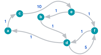
In this example graph, a number over an edge indicates its weight.
Solution
Closeness centrality scores for each node \(x\), denoted \(CC_x\):
- \(CC_a \approx 0.102\), \(CC_b \approx 0.2\), \(CC_c \approx 0.087\)
- \(CC_d \approx 0.151\), \(CC_e \approx 0.454\), \(CC_f \approx 0.151\)
Algorithm details
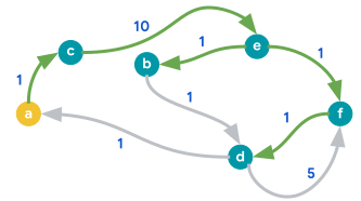
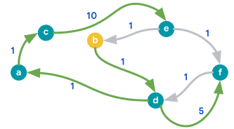
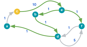
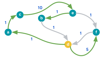
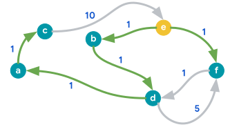
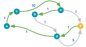
The algorithm computes the shortest-path distances for all nodes in the graph (represented in the following diagrams as green edges for each source node \(x\)), as well as the set of nodes \(R(x)\) that each node \(x\) can reach:
Node \(a\):
- Shortest-path distances: $\{b: 12, c: 1, d: 13, e: 11, f: 12\}$
- $R(a) = \{b, c, d, e, f\}$
Node \(b\):
- Shortest-path distances: $\{a: 2, c: 3, d: 1, e: 13, f: 6\}$
- $R(b) = \{a, c, d, e, f\}$
Node \(c\):
- Shortest-path distances: $\{a: 13, b: 11, d: 12, e: 10, f: 11\}$
- $R(c) = \{a, b, d, e, f\}$
Node \(d\):
- Shortest-path distances: $\{a: 1, b: 13, c: 2, e: 12, f: 5\}$
- $R(d) = \{a, b, c, e, f\}$
Node \(e\):
- Shortest-path distances: $\{a: 3, b: 1, c: 4, d: 2, f: 1\}$
- $R(e) = \{a, b, c, d, f\}$
Node \(f\):
- Shortest-path distances: $\{a: 2, b: 14, c: 3, d: 1, e: 13\}$
- $R(f) = \{a, b, c, d, e\}$
For every node \(x\), the sum of the shortest-path distances between \(x\) and each other node \(y\) reachable from it in the graph is computed as follows, using the shortest-path distances computed earlier (each summation takes \(y\) in alphabetical order):
- Node a: \(\sum_{y \in R(a)} d(a,y) = 12 + 1 + 13 + 11 + 12 = 49\)
- Node b: \(\sum_{y \in R(b)} d(b,y) = 2 + 3 + 1 + 13 + 6 = 25\)
- Node c: \(\sum_{y \in R(c)} d(c,y) = 13 + 11 + 12 + 10 + 11 = 57\)
- Node d: \(\sum_{y \in R(d)} d(d,y) = 1 + 13 + 2 + 12 + 5 = 33\)
- Node e: \(\sum_{y \in R(e)} d(e,y) = 3 + 1 + 4 + 2 + 1 = 11\)
- Node f: \(\sum_{y \in R(f)} d(f,y) = 2 + 14 + 3 + 1 + 13 = 33\)
Given these values, \(CC_x\) can be computed for every node \(x\) in the graph:
\[ \begin{align*} CC_a &= |R(a)| / \sum_{y \in R(a)} d(a, y) = 5 / 49 \approx 0.102 \\ CC_b &= |R(b)| / \sum_{y \in R(b)} d(b, y) = 5 / 25 = 0.2 \\ CC_c &= |R(c)| / \sum_{y \in R(c)} d(c, y) = 5 / 57 \approx 0.087 \\ CC_d &= |R(d)| / \sum_{y \in R(d)} d(d, y) = 5 / 33 \approx 0.151 \\ CC_e &= |R(e)| / \sum_{y \in R(e)} d(e, y) = 5 / 11 \approx 0.454 \\ CC_f &= |R(f)| / \sum_{y \in R(f)} d(f, y) = 5 / 33 \approx 0.151 \end{align*} \]
Example 2
Input graph
This example illustrates the computation of the (standard) closeness centrality and the Wasserman-Faust closeness centrality. This is similar to Example 1, except that the edge \(da\) is not present. Note that with this change the graph is no longer strongly connected. The following results show that the standard closeness centralities and the Wasserman-Faust closeness centralities are different.
Consider the following input graph:
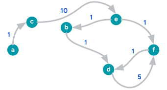
In this example graph, a number over an edge indicates its weight.
Solution
Standard closeness centrality scores for each node \(x\), denoted \(CC_x\):
- \(CC_a \approx 0.102\), \(CC_b \approx 0.285\), \(CC_c \approx 0.090\)
- \(CC_d = 0.2\), \(CC_e = 0.75\), \(CC_f = 1\)
Wasserman-Faust closeness centrality scores for each node \(x\), denoted \(CC^{WF}_x\):
- \(CC^{WF}_a \approx 0.102\), \(CC^{WF}_b \approx 0.114\), \(CC^{WF}_c \approx 0.072\)
- \(CC^{WF}_d \approx 0.04\), \(CC^{WF}_e \approx 0.45\), \(CC^{WF}_f \approx 0.2\)
Algorithm details
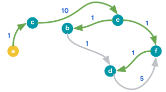
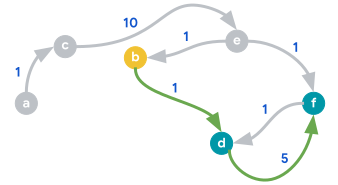
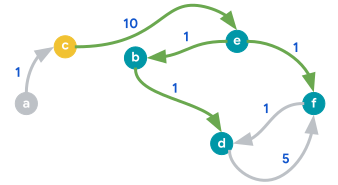
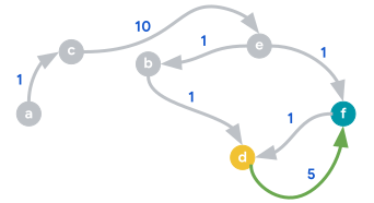
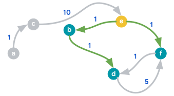
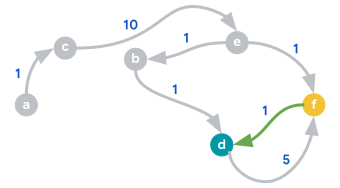
The algorithm computes the shortest-path distances for all nodes in the graph (represented in the following diagrams as green edges for each source node \(x\)), as well as the set of nodes \(R(x)\) that each node \(x\) can reach:
Node \(a\):
- Shortest-path distances: $\{b: 12, c: 1, d: 13, e: 11, f: 12\}$
- $R(a) = \{b, c, d, e, f\}$
Node \(b\):
- Shortest-path distances: $\{d: 1, f: 6\}$
- $R(b) = \{d, f\}$
Node \(c\):
- Shortest-path distances: $\{b: 11, d: 12, e: 10, f: 11\}$
- $R(c) = \{b, d, e, f\}$
Node \(d\):
- Shortest-path distances: $\{f: 5\}$
- $R(d) = \{f\}$
Node \(e\):
- Shortest-path distances: $\{b: 1, d: 2, f: 1\}$
- $R(e) = \{b, d, f\}$
Node \(f\):
- Shortest-path distances: $\{d: 1\}$
- $R(f) = \{d\}$
For every node \(x\), the sum of the shortest-path distances between \(x\) and each other node \(y\) reachable from it in the graph is computed as follows, using the shortest-path distances computed earlier (each summation takes \(y\) in alphabetical order):
- Node a: \(\sum_{y \in R(a)} d(a,y) = 12 + 1 + 13 + 11 + 12 = 49\)
- Node b: \(\sum_{y \in R(b)} d(b,y) = 1 + 6 = 7\)
- Node c: \(\sum_{y \in R(c)} d(c,y) = 11 + 12 + 10 + 11 = 44\)
- Node d: \(\sum_{y \in R(d)} d(d,y) = 5\)
- Node e: \(\sum_{y \in R(e)} d(e,y) = 1 + 2 + 1 = 4\)
- Node f: \(\sum_{y \in R(f)} d(f,y) = 1\)
Given these values, the standard closeness centrality \(CC_x\) for every node \(x\) in the graph is computed as follows:
\[ \begin{align*} CC_a &= |R(a)| / \sum_{y \in R(a)} d(a, y) = 5 / 49 \approx 0.102 \\ CC_b &= |R(b)| / \sum_{y \in R(b)} d(b, y) = 2 / 7 \approx 0.285 \\ CC_c &= |R(c)| / \sum_{y \in R(c)} d(c, y) = 4 / 44 \approx 0.090 \\ CC_d &= |R(d)| / \sum_{y \in R(d)} d(d, y) = 1 / 5 = 0.2 \\ CC_e &= |R(e)| / \sum_{y \in R(e)} d(e, y) = 3 / 4 = 0.75 \\ CC_f &= |R(f)| / \sum_{y \in R(f)} d(f, y) = 1 / 1 = 1 \end{align*} \]
Using the standard closeness centralities, the Wasserman-Faust closeness centrality \(CC^{WF}_x\) for every node \(x\) in the graph is computed as follows:
\[ \begin{align*} CC^{WF}_a &= CC_a * |R(a)| / (n-1) = CC_a * 5 / (6-1) \approx 0.102 \\ CC^{WF}_b &= CC_b * |R(b)| / (n-1) = CC_b * 2 / (6-1) \approx 0.114 \\ CC^{WF}_c &= CC_c * |R(c)| / (n-1) = CC_c * 4 / (6-1) \approx 0.072 \\ CC^{WF}_d &= CC_d * |R(d)| / (n-1) = CC_d * 1 / (6-1) = 0.04 \\ CC^{WF}_e &= CC_e * |R(e)| / (n-1) = CC_e * 3 / (6-1) = 0.45 \\ CC^{WF}_f &= CC_f * |R(f)| / (n-1) = CC_f * 1 / (6-1) = 0.2 \end{align*} \]
External references
- The definition of Wasserman-Faust closeness centrality was introduced in Social Network Analysis (Cambridge University Press, 1994).
- The
HYBRIDalgorithm was introduced in Computing Classic Closeness Centrality, at Scale (Conference on Online Social Networks, 2014).