

This algorithm computes the betweenness centralities of all nodes of a directed graph with positive edge weights, defined as follows. Let \(V\) be the set of all nodes in the graph. For any pair of distinct nodes \(x\) and \(y\), define the following notation:
- \(P(x, y)\) is the set of all shortest paths from node \(x\) to node \(y\).
- \(\delta_{xy}(z)\), where \(z\) is a node other than \(x\) and \(y\), is the pair-dependency of nodes \(x\) and \(y\) on \(z\). This quantity represents the fraction of shortest paths from \(x\) to \(y\) that pass through \(z\) (or zero if \(x\) is not reachable from \(y\)):
\[ \delta_{xy}(z) = \begin{cases} \frac{|\{p \in P(x, y) : z \in p\}|}{|P(x, y)|} & \text{, if } y \text{ is reachable from } x ;\\ 0 & \text{, otherwise.}\\ \end{cases} \]
The betweenness centrality of node \(z\) is the sum of the pair-dependencies of all pairs of nodes (other than \(z\) itself) on \(z\):
\[ \text{betweenness_centrality}(z) = \sum_{x, y \in V \setminus \{z\} : x \neq y} \delta_{xy}(z). \]
Note that the betweenness centrality of a node is always between \(0\) and \((|V| - 1) \cdot (|V| - 2)\), inclusive.
The algorithm also supports an approximate, source-constrained mode, where it computes pair-dependencies only for source nodes \(x\) in some set of source nodes \(S\) (a subset of \(V\)) that the algorithm samples:
\[ \text{betweenness_centrality}_S(z) = \sum_{x \in S \setminus \{z\} , y \in V \setminus \{x, z\}} \delta_{xy}(z). \]
Note that the approximate betweenness centrality of a node is always between \(0\) and \(|S| \cdot (|V| - 2)\), inclusive. Moreover, the exact betweenness centrality is a special case of the approximate betweenness centrality with \(S\) equal to \(V\).
Interface specifications
The following list summarizes the expectations on the graph passed as input to this algorithm. These expectations complement the ones listed in General assumptions on input graphs.
- Directed graph (an undirected graph can be converted into a directed graph by replacing each undirected edge \(xy\) with two directed edges \(xy\) and \(yx\), both with the same weight as the original edge).
- Edge weights: Must be positive. The output is a list of \(|V|\) floating-point numbers, corresponding to the betweenness centralities of all nodes.
The following parameters configure the algorithm:
| Name | Type | Description |
|---|---|---|
num_source_nodes
|
integer (optional) | If set, must be positive, and
specifies how many source nodes
the algorithm should select for
computing approximate betweenness
centralities. If not set, or set
to a number larger than the number
of nodes in the graph, then the
algorithm uses all nodes as source
nodes, that is, the algorithm
computes exact centralities.
Higher values lead to better approximations, but also to longer running times. |
sampling_seed
|
integer (optional) | The seed for the random number
generator that the algorithm uses
to select the source nodes (if
num_source_nodes is set). The
algorithm selects the same set of
source nodes when given the same
input graph, num_source_nodes,
and sampling_seed. |
Algorithm
The algorithm starts by selecting which nodes it uses as source nodes. If
num_source_nodes is not set, then the algorithm considers all nodes source nodes. If
num_source_nodes is set, then the algorithm attempts to select this many
source nodes, using reservoir sampling (without replacement). At each sampling
step, the probability of selecting a given node that the algorithm has not yet selected
is proportional to its out-degree. The algorithm never selects nodes with out-degree zero. If the number of nodes with positive out-degree is smaller than
num_source_nodes (in particular, this happens if num_source_nodes is larger
than the number of nodes in the graph), then the algorithm will use all nodes
with positive out-degree as source nodes (note that this means that the
algorithm will compute exact betweenness centralities).
For each source node \(x\) (in parallel), the algorithm then runs a parallel single-source shortest path (SSSP) algorithm to compute the shortest-path distances \(d(x, y)\) from \(x\) to all other nodes \(y\). Then it computes the number of shortest paths from \(x\) to any other node \(y\), by observing that \(|P(x, x)| = 1\) and for any node \(y \neq x\) that can be reached from \(x\), the following recurrence relation holds:
\[ |P(x, y)| = \sum_{z \in V : zy \in E, d(x, z) + w_{zy} = d(x, y)} |P(x, z)| , \]
where \(w_{zy}\) denotes the weight of edge \(zy\).
The algorithm then computes the contribution of the source node \(x\) to the betweenness centrality of each other node \(z\), namely
\[ \delta_{x\odot}(z) := \sum_{y \in V \setminus \{x, z\} } \delta_{xy}(z) , \]
using the fact that \(\delta_{x\odot}(x) = 0\) and for any other node \(z \neq x\) that can be reached from \(x\), the following recurrence relation holds:
\[ \delta_{x\odot}(z) = \sum_{y \in V : zy \in E, d(x, z) + w_{zy} = d(x, y)} \frac{|P(x,z)|}{|P(x,y)|}( 1+ \delta_{x\odot}(y) ) . \]
Finally, the algorithm adds up the contributions from all source nodes to obtain the final (exact or approximate) betweenness centralities.
Because the edges in the input graph have positive weights, the preceding recurrence relations don't introduce cyclic dependencies.
Computational complexity
The algorithm is a parallel algorithm that runs in \(O(sm\log n)\) work and
\(O(m\log n)\) depth, where \(n\) and \(m\) denote the number of nodes and edges
in the input graph, respectively, and \(s\) denotes the number of source nodes
that the algorithm uses (which is at most num_source_nodes if that parameter is set, or \(n\) otherwise).
The algorithm uses \(O(\text{num_threads} \cdot n)\) memory, where \(\text{num_threads}\) is the number of threads that the algorithm uses during execution.
Example
This example illustrates the computation of the exact betweenness centrality for a specific node.
Input graph
Consider the following input graph:
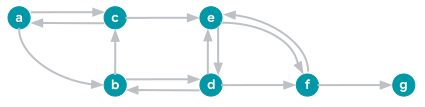
For the provided graph, assume that the weight of each edge is 1.0.
Solution
Betweenness centrality scores for each node x in the graph, denoted \(BC_x\):
- \(BC_a\) = 1.0, \(BC_b\) = 8.0, \(BC_c\) = 6.5, \(BC_d = 9.5\)
- \(BC_e\) = 8.0, \(BC_f\) = 5.0, \(BC_g\) = 0.0
Algorithm details
Recall that betweenness centrality measures a node's centrality by determining how often it lies on the shortest paths between all other pairs of distinct nodes in the graph.
Instead of detailing all the calculations for all the nodes and respective pairs, this section focuses on a specific example to illustrate the algorithm's process. Assume the goal is to calculate the betweenness centrality for node \(d\) (colored in yellow), denoted by \(BC_d\).
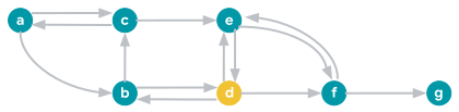
If all the shortest paths between node \(x\) and node \(y\) bypass node \(d\), it means node \(d\) is not needed as an intermediary for that specific connection. Consequently, the pair-dependency of the pair \((x, y)\) on node \(d\) is 0.
For example, tracing all the shortest paths between pairs of nodes like \((a, b)\), \((a, e)\), or \((e, g)\) reveals that node \(d\) is not on any of them. That means those pairs of nodes don't contribute to node \(d\)'s betweenness centrality. In this particular example, there are 19 such pairs.
Formally, the pair dependency of a pair \((x, y)\) on \(d\) is the total number of shortest paths between \((x, y)\) passing through \(d\), divided by the total number of shortest paths between \((x, y)\).
Consider the pairs of nodes for which the pair-dependency on node \(d\) is not 0:
pair (a, f): There are two shortest paths, one of which passes through node \(d\) (solid dark blue edges) and one of which doesn't (dashed light blue edges):

The pair-dependency is therefore 0.5 (that is, 1/2).
pair (a, g): Again, there are two shortest paths, one of which passes through node \(d\):

The pair-dependency is therefore 0.5 (that is, 1/2).
pair (b, e): Here again there are two shortest paths, one of which passes through node \(d\):

The pair-dependency is therefore 0.5 (that is, 1/2).
pair (b, f): In this case there is a unique shortest path, and it passes through node \(d\):

The pair-dependency is thus 1.0 (that is, 1/1).
pair (b, g): There is a unique shortest path, and it passes through node \(d\):

The pair-dependency is thus 1.0 (that is, 1/1).
pair (e, a): There is a unique shortest path, and it passes through node \(d\):

The pair-dependency is 1.0 (that is, 1/1).
pair (e, b): There is a unique shortest path, and it passes through node \(d\):

The pair-dependency is 1.0 (that is, 1/1).
pair (e, c): There is a unique shortest path, and it passes through node \(d\):

The pair-dependency is 1.0 (that is, 1/1).
pair (f, a): There is a unique shortest path, and it passes through node \(d\):

The pair-dependency is 1.0 (that is, 1/1).
pair (f, b): There is a unique shortest path, and it passes through node \(d\):

The pair-dependency is 1.0 (that is, 1/1).
pair (f, c): There is a unique shortest path, and it passes through node \(d\):

The pair-dependency is 1.0 (that is, 1/1).
Finally, summing the pair-dependencies of the 11 node pairs on node \(d\) yields:
\[BC_d = (3 * 0.5) + (8 * 1.0) = 9.5\]
A similar computation yields the betweenness centralities of all other nodes.
External references
- The algorithm is based on Brandes' algorithm, introduced in A Faster Algorithm for Betweenness Centrality (Journal of Mathematical Sociology, 2001). In particular, that paper introduced the recurrence relations.
- While Brandes' algorithm is a sequential algorithm, the implementation described in this page leverages parallelism, following the approach from Ligra: A Lightweight Graph Processing Framework for Shared Memory (Principles and Practice of Parallel Programming, 2013).
- An earlier version of the algorithm, which handles the single-source case only and requires the graph to be unweighted, was described and benchmarked in Theoretically Efficient Parallel Graph Algorithms Can Be Fast and Scalable (Symposium on Parallelism in Algorithms and Architectures, 2018). An open-source implementation of that earlier version is available on the Graph Based Benchmark Suite (GBBS).