Modularity clustering

This algorithm computes a non-overlapping clustering of an undirected graph with non-negative edge weights, heuristically trying to maximize the modularity score, defined as follows. Let

• \(\deg(x)\) be the weighted degree of node \(x\) in the graph, that is, the sum of the weights of all edges incident to \(x\).
• \(M\) be the sum of all weighted node degrees. In the case of an unweighted graph without self-loops, this is exactly twice the number of undirected edges in the graph.
• \(w_{xy}\) be the weight of the edge \(xy\) in the graph, or \(0\) if there is no such edge. The graph must be undirected, so \(w_{xy}\) and \(w_{yx}\) must be equal.
• \(r\) be a non-negative resolution parameter, which controls the granularity of the clustering. Smaller resolution values tend to lead to larger clusters.
• \(C\) be the set of all clusters in the clustering. Each cluster is a set of nodes, and each node is contained in exactly one cluster.

Then, the modularity score is defined as follows.

\[ \sum_{c \in C} \sum_{x, y \in c} w_{xy} - \frac{r \cdot \deg(x) \cdot \deg(y)}{M} \]

The second sum goes over all unordered pairs of nodes in a cluster exactly once. In particular: the algorithm considers each undirected edge, including a self-loop, exactly once.

Other definitions of modularity

Note that there are multiple definitions of modularity. However, most of them are equivalent from the optimization perspective, as they are monotone in each other. In particular, the algorithm uses an objective that is \(M\) times the modularity score as Wikipedia defines.

Interface specifications

The following list summarizes the expectations on the graph passed as input to this algorithm. These expectations complement the ones listed in General assumptions on input graphs.

• Undirected graph
• Edge weights: Must be non-negative.

The output is a non-overlapping clustering, with the best modularity score that the algorithm achieves for the given resolution parameter \(r\).

The following parameters configure the algorithm:

Name	Type	Description
resolution	floating-point number	Controls the granularity of the clustering. Must be finite and non-negative. Smaller resolution values tend to lead to larger clusters. Typical values are in the range [0.5, 5]. The most frequently used value is 1. When the resolution is zero, the algorithm (with a sufficient number of iterations) finds the connected components of the graph (ignoring edges whose weight is zero).
num_iterations	integer	Maximum number of outer iterations of the algorithm. Must be positive. Larger values tend to lead to higher-quality clusterings (w.r.t. the objective function), but also tend to increase the running time.
num_inner_iterations	integer	Maximum number of inner iterations of the algorithm. Must be positive. Larger values tend to lead to higher-quality clusterings (w.r.t. the objective function), but also tend to increase the running time.

Algorithm

The underlying algorithm is a parallel, asynchronous implementation of the Louvain method.

The algorithm runs a sequence of outer iterations (or just iterations, for short). In the first outer iteration, the algorithm starts by assigning each node to a cluster of its own. Then, in each inner iteration of the algorithm, the algorithm considers each node \(x\), in parallel. If moving \(x\) to a different cluster increases the modularity objective, the algorithm moves it to a cluster that maximizes the objective increase; otherwise, the algorithm does not move \(x\). The algorithm repeats the inner iterations until no nodes move or it reaches the maximum number of inner iterations.

Once the algorithm completes the inner iterations, it contracts each cluster to a single node and starts a new outer iteration on the contracted graph, as described in the preceding section—that is, the algorithm assigns each node in the contracted graph to its own cluster, then performs a sequence of inner iterations. The contracted graph is defined as follows:

• The weight of each node in the contracted graph is the total weight of the nodes that formed it.

• An edge \(xy\) exists in the contracted graph if and only if any edge existed between a node in the cluster corresponding to \(x\) in the original graph and a node in the cluster corresponding to \(y\) in the original graph.

• The weight of an edge \(xy\) in the contracted graph is the sum of the weights of all edges in the original graph that the algorithm contracted into it.

For a node \(v\) in the contracted graph corresponding to a cluster \(c\) in the original graph, moving \(v\) to a new cluster in the contracted graph is equivalent to moving all nodes in \(c\) to a new cluster in the original graph.

The outer iterations continue until convergence to a local optimum (that is, until the algorithm cannot move any node from its current cluster to a different one at the start of an outer iteration while increasing the objective) or until the algorithm reaches the maximum number of outer iterations.

Note: The algorithm is non-deterministic because:

• the order in which the algorithm processes nodes within each inner iteration may affect the final clustering; and
• the algorithm processes the nodes in parallel, leading to a non-deterministic ordering.

Computational complexity

The algorithm is a parallel algorithm that runs in \(O(\text{num_iterations} \cdot \text{num_inner_iterations}\cdot m)\) work and \(O(\text{num_iterations} \cdot \text{num_inner_iterations}\cdot \log n)\) depth, where \(n\) and \(m\) denote the number of nodes and edges in the input graph, respectively, and \(\text{num_iterations}\) and \(\text{num_inner_iterations}\) denote the number of (outer) iterations and inner iterations, respectively. Running the algorithm on a machine that supports high amounts of parallelism tends to lead to a smaller running time.

The algorithm uses \(O(m + n)\) memory.

Example

Note: This example uses a sequential algorithm for illustration purposes, while in the actual implementation the algorithm executes some parts in parallel.

Input graph

Consider the following input graph:

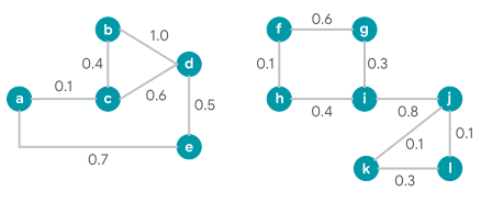
The following description assumes that the resolution parameter \(r\) is 1.

Solution

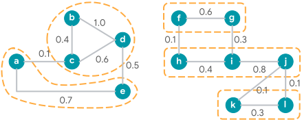
The modularity score is the sum of modularity increases that the algorithm obtained in the outer iterations (in this case, the algorithm performed a single outer iteration where it executed moves):

\[\text{Modularity Score} = \Delta \text{Modularity}_1 \approx 3.860\]

This is a clustering optimizing the objective, but in general the algorithm may find a suboptimal solution.

Algorithm details

Initially, the algorithm assigns each node to a cluster of its own (represented in the diagram with orange dashes):

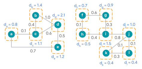
The algorithm computes the weighted degree of node \(x\), represented by \(d_x\).

The sum of all weighted node degrees is \(M = 12.0\).

\[\text{Modularity Score} = 0\]

Outer iteration #1 - inner iteration #1

The algorithm iterates over all nodes in some order. For each node \(x\), the algorithm moves \(x\) to a cluster (either the cluster of a neighbor of \(x\), or a brand new cluster containing just \(x\) itself) chosen such that the increase in the modularity score is maximized and positive.

Note: The resulting cluster formations depend on the order of best move consideration. This example assumes that the algorithm processes the nodes in alphabetical order. In the implementation, this order is non-deterministic.

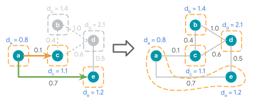
The following are the possible moves for each node (\(x\)) in the left component of the graph and their effect on the modularity score—where a red arrow indicates no increase, an orange arrow indicates an increase but not the highest one for that node, and a green arrow indicates that node's best move, if there is a move that increases the modularity score.

Let \(\Delta \text{Modularity}_1\) denote the overall modularity increase achieved in the outer iteration #1. Initially, \(\Delta \text{Modularity}_1 = 0\), and the algorithm updates it each time it executes a move.

Node (a):

Node (a)'s possible moves, and their effect on the modularity score:

• (a) \(\rightarrow\) (c): 0.1 - 10.81.1/12 \(\approx\) 0.027
• (a) \(\rightarrow\) (e): 0.7 - 10.81.2/12 = 0.620

The move to cluster (e) maximizes the increase of the modularity score.

\[\Delta \text{Modularity}_1 = 0 + 0.620 = 0.620\]

Node (b):

Node (b)'s possible moves, and their effect on the modularity score:

• (b) \(\rightarrow\) (c): 0.4 - 11.41.1/12 \(\approx\) 0.272
• (b) \(\rightarrow\) (d): 1.0 - 11.42.1/12 = 0.755

The move to cluster (d) maximizes the increase of the modularity score.

\[\Delta \text{Modularity}_1 = 0.620 + 0.755 = 1.375\]

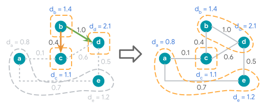
Node (c):

Node (c)'s possible moves, and their effect on the modularity score:

• (c) \(\rightarrow\) (ae): 0.1 - 11.1(0.8+1.2)/12 \(\approx\) -0.083
• (c) \(\rightarrow\) (bd): (0.4+0.6) - 11.1(1.4+2.1)/12 \(\approx\) 0.680

The move to cluster (bd) maximizes the increase of the modularity score.

\[\Delta \text{Modularity}_1 \approx 1.375 + 0.680 = 2.055\]

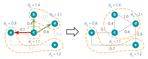
Node (d):

Node (d)'s possible moves, and their effect on the modularity score:

• split from (bc): -(1.0+0.6) + 12.1(1.4+1.1)/12 \(\approx\) -1.162
• (d) \(\rightarrow\) (ae): -1.162 + 0.5 - 12.1(0.8+1.2)/12 \(\approx\) -1.012

No move increases the modularity score, so the algorithm commits no move.

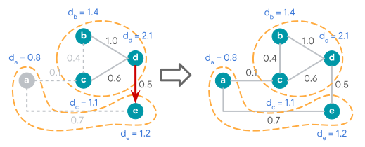
Node (e):

Node (e)'s possible moves, and their effect on the modularity score:

• split from (a): -0.7 + 11.20.8/12 = -0.620
• (e) \(\rightarrow\) (bcd): -0.620 + 0.5 - 11.2(1.4+1.1+2.1)/12 = -0.580

No move increases the modularity score, so the algorithm commits no move.

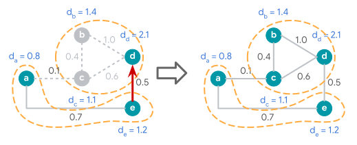
Running similar steps on the right component of the graph, the algorithm executes the moves (f) \(\rightarrow\) (g), (h) \(\rightarrow\) (i), (i) \(\rightarrow\) (j), and (k) \(\rightarrow\) (l), thus producing clusters (fg), (h), (ij), and (kl). The algorithm updates \(\Delta \text{Modularity}_1\) to account for those 4 additional moves:

\[ \begin{align*} \Delta \text{Modularity}_1 &\approx 2.055 &\text{// previous value} \\ &+ (0.6 - 1*0.7*0.9/12) &\text{// (f)} \rightarrow \text{(g)} \\ &+ (0.4 - 1*0.5*1.5/12) &\text{// (h)} \rightarrow \text{(i)} \\ &+ (-0.4 + 1*0.5*1.5/12 + 0.8 - 1*1.5*1.0/12) &\text{// (i)} \rightarrow \text{(j)} \\ &+ (0.3 - 1*0.4*0.4/12) &\text{// (k)} \rightarrow \text{(l)} \\ &\approx 3.564 \end{align*} \]

Outer iteration #1 - inner iteration #2

The algorithm starts a new inner iteration to check for moves that increase the modularity score. Only one such move exists, for node (h) (omitting other calculations for brevity).

Node (h):

Node (h)'s possible moves, and their effect on the modularity score:

• (h) \(\rightarrow\) (fg): 0.1 - 10.5(0.7+0.9)/12 \(\approx\) 0.033
• (h) \(\rightarrow\) (ij): 0.4 - 10.5(1.5+1.0)/12 \(\approx\) 0.296

The move to cluster (ij) maximizes the increase of the modularity score.

\[\Delta \text{Modularity}_1 \approx 3.564 + 0.296 = 3.860\]

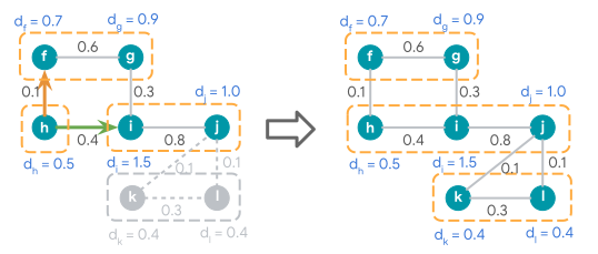
Recall that the algorithm repeats the inner iterations until no nodes move or it reaches the maximum number of inner iterations (by default, 10). Hence, the algorithm would perform a third inner iteration. In this specific case no single-node move increases the modularity score, and so the algorithm commits no additional move. Since no moves occur in an inner iteration, the algorithm contracts the graph.

Contracted Graph

Here's the result of contracting the graph:

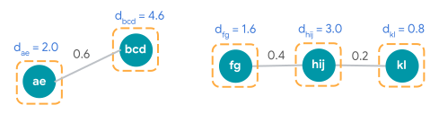
The weight of an edge \(xy\) in the contracted graph is the sum of the weights of all edges of the original graph that the algorithm contracted into it.

The weighted degree \(d_x\) of each node \(x\) in the contracted graph is equal to the sum of the weighted degrees of its nodes. For example \(d_{bcd} = d_b + d_c + d_d = 1.4 + 1.1 + 2.1 = 4.6\).

Outer iteration #2 - inner iteration #1

The algorithm considers each cluster in the contracted graph.

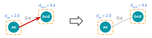
Cluster (ae):

Cluster (ae)'s only possible move, and its effect on the modularity score:

• (ae) \(\rightarrow\) (bcd): 0.6 - 12.04.6/12 \(\approx\) -0.166

This move does not increase the modularity score, so the algorithm does not commit it.

Cluster (fg):

Cluster (fg)'s only possible move, and its effect on the modularity score:

• (fg) \(\rightarrow\) (hij): 0.4 - 11.63.0/12 = 0

This move does not increase the modularity score, so the algorithm does not commit it.

Cluster (hij):

Cluster (hij)'s possible moves, and their effect on the modularity score:

• (hij) \(\rightarrow\) (fg): 0.4 - 13.01.6/12 = 0
• (hij) \(\rightarrow\) (kl): 0.2 - 13.00.8/12 = 0

No move increases the modularity score, so the algorithm commits no move.

Cluster (kl):

Cluster (kl)'s only possible move, and its effect on the modularity score:

• (kl) \(\rightarrow\) (hij): 0.2 - (10.83.0)/12 = 0

This move does not increase the modularity score, so the algorithm does not commit it.

At this point, there is no single-node move that would increase the modularity score. Since the algorithm committed no move in this outer iteration, it terminates, producing the clusters (ae), (bcd), (fg), (hij), and (kl).

External references

• The modularity measure was introduced in Finding and Evaluating Community Structure in Networks (Physical Review E, 2004).
• This algorithm was introduced in Scalable Community Detection via Parallel Correlation Clustering (Proceedings of the VLDB Endowment, 2021).
• The algorithm was benchmarked in The ParClusterers Benchmark Suite (PCBS): A Fine-Grained Analysis of Scalable Graph Clustering (Proceedings of the VLDB Endowment, 2025).
• An open-source implementation is available on GitHub.