

This algorithm computes a clustering of an undirected graph with non-negative edge weights based on the majority-vote label propagation algorithm. Label propagation works by repeatedly recomputing the labels of nodes that are active by identifying, for each such node, the label with the largest total weight in its neighborhood. If a node is active and changes its label in one iteration, the algorithm marks all of its neighbors to be active in the next iteration, so that they have a chance to change their labels. After the final iteration, the algorithm groups nodes with equal labels into clusters.
Interface specifications
The following list summarizes the expectations on the graph passed as input to this algorithm. These expectations complement the ones listed in General assumptions on input graphs.
- Undirected graph
- Edge weights: Must be non-negative.
The algorithm also admits as input a list of seed labels (that is, non-negative integer labels for some of the nodes in the graph), which the algorithm uses to initialize the labels of the nodes at the very beginning of the algorithm (before the execution of the first iteration). Note that the algorithm may update the labels of such nodes throughout its execution, so at the end they need not be equal to the provided seed labels. Nodes without a seed label receive an initial label that the algorithm chooses, which is different from the initial labels of all other nodes.
The output of the algorithm is a non-overlapping clustering. The algorithm assigns each node to a single cluster corresponding to its final label.
The following parameters configure the algorithm:
| Name | Type | Description |
|---|---|---|
num_iterations
|
integer | The maximum number of iterations of label propagation that the algorithm performs. Must be finite and positive. |
Algorithm
The algorithm executes a sequence of up to num_iterations iterations. Before
the first iteration, the algorithm computes the initial labels as follows:
- For each node with a seed label, the algorithm sets the initial label of the node to its seed label.
- For each other node, the algorithm assigns an initial label that is different from the initial labels of all the other nodes.
The algorithm then marks all nodes that have at least one neighbor as active,
and starts the sequence of up to num_iterations iterations. Within each
iteration, each active node \(x\) computes a new label for itself. The new label
is the label that appears with the highest weight in its neighborhood. The
algorithm computes the weight of a label by summing the weights of all edges that connect
\(x\) with a neighbor that has that label. If two labels appear with the same
weight, the algorithm breaks ties in favor of the label with the higher ID. Note that the
label of the node in the next iteration is independent of its current label. The
new label for node \(x\) may or may not differ from the label it
had prior to the beginning of the iteration; if it differs, then the
algorithm marks all neighbors of \(x\) as active for the following
iteration. Once the algorithm processes all active nodes, it proceeds to the
next iteration. The algorithm stops once there are no more active nodes, or once
it has executed num_iterations iterations.
Parallel implementations of the majority vote label propagation algorithm typically rely on locks to handle concurrent access and updates of the label of a node from multiple threads within each iteration. Lock contention can significantly increase the running time; moreover, performing label updates within each iteration in a non-deterministic order leads to non-deterministic results. To address those issues, and obtain a lock-free and deterministic algorithm, the algorithm uses a graph coloring algorithm. At the very start of the algorithm (before executing the first iteration), the algorithm computes a coloring of the input graph, that is, it assigns a color to each of its nodes, in such a way that no two adjacent nodes have the same color. The coloring algorithm attempts to use a small number of colors, using the largest-log-degree-first (LLF) heuristic. Within each iteration, the implementation of the majority vote label propagation algorithm processes the color classes one at a time: for each color (sequentially, and in a deterministic order), it updates the labels of all nodes that have that color in parallel.
Computational complexity
The algorithm is a parallel algorithm that runs in \(O(\text{num_iterations}\cdot (m+n))\) work and \(O(\text{num_iterations}\cdot \Delta \log n)\) depth, where \(n\) and \(m\) denote the number of nodes and edges in the input graph, respectively, \(\text{num_iterations}\) denotes the number of iterations, and \(\Delta\) denotes the maximum degree of a node in the input graph. Running the algorithm on a machine that supports high amounts of parallelism tends to lead to a smaller running time.
The algorithm uses \(O(m+n)\) memory.
Examples
Example 1
Input graph
Consider the following input graph:
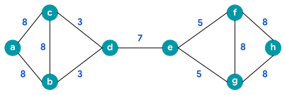
For the provided undirected weighted graph, assume the following:
- The number of iterations is 10.
- A number over an edge indicates its weight.
- The input does not contain seed labels.
Solution
This graph shows the final labels that the algorithm produces. The notation \(L_x\) next to a node \(x\) indicates its label. The nodes are color-coded according to their labels.
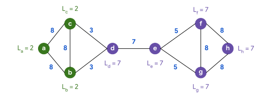
Note: the resulting labels depend on the order of node processing. This example assumes for simplicity that in each iteration the algorithm processes the active nodes in alphabetical order. In the actual implementation, this order is deterministic, but unspecified.
Algorithm details
If the input does not provide labels, the algorithm starts by assigning a distinct initial label to each node. Here, the algorithm assigns initial labels 0, 1, 2, ..., 7 in alphabetical order.
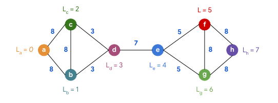
The algorithm marks all nodes as active for the first iteration.
Iteration #0: The algorithm processes the active nodes [\(a, b, c, d, e, f, g, h\)] in that order.
Processing node \(a\), with \(L_a\) = 0:
- Weight that each label gets:
- 1: 8 (all from node \(b\))
- 2: 8 (all from node \(c\))
- The algorithm assigns label 2 to node \(a\).
- Note: the algorithm breaks ties by choosing the largest label among the ones with highest weight.

Processing node \(b\), with \(L_b\) = 1:
- Weight that each label gets:
- 2: 16 (8 from node \(a\), and 8 from node \(c\))
- 3: 3 (all from node \(d\))
- The algorithm assigns label 2 (the label with the highest weight) to node \(b\).

Processing node \(c\), with \(L_c\) = 2:
- Weight that each label gets:
- 2: 16 (8 from node \(a\), and 8 from node \(b\))
- 3: 3 (all from node \(d\))
- The algorithm assigns label 2 (the label with the highest weight) to node \(c\).

Processing node \(d\), with \(L_d\) = 3:
- Weight that each label gets:
- 2: 6 (3 from node \(b\), and 3 from node \(c\))
- 4: 7 (all from node \(e\))
- The algorithm assigns label 4 (the label with the highest weight) to node \(d\).

Processing node \(e\), with \(L_e\) = 4:
- Weight that each label gets:
- 4: 7 (all from node \(d\))
- 5: 5 (all from node \(f\))
- 6: 5 (all from node \(g\))
- The algorithm assigns label 4 (the label with the highest weight) to node \(e\).

Processing node \(f\), with \(L_f\) = 5:
- Weight that each label gets:
- 4: 5 (all from node \(e\))
- 6: 8 (all from node \(g\))
- 7: 8 (all from node \(h\))
- The algorithm assigns label 7 to node \(f\)
- Note: the algorithm breaks ties by choosing the largest label among the ones with highest weight.

Processing node \(g\), with \(L_g\) = 6:
- Weight that each label gets:
- 4: 5 (all from node \(e\))
- 7: 16 (8 from node \(f\), and 8 from node \(h\))
- The algorithm assigns label 7 (the label with the highest weight) to node \(g\).

Processing node \(h\), with \(L_h\) = 7:
- Weight that each label gets:
- 7: 16 (8 from node \(f\), and 8 from node \(g\))
- The algorithm assigns label 7 (the label with the highest weight) to node \(h\).

Here's the assignment of labels at the end of iteration #0:

- Nodes whose labels have changed: [\(a, b, d, f, g\)]
- Active nodes (neighbors of nodes with changed labels): [\(a, b, c, d, e, f, g, h\)]
Iteration #1: The algorithm processes the active nodes [\(a, b, c, d, e, f, g, h\)], in that order. Since the preceding iteration shows an identical process, this example does not show the detailed steps for each node from here on.
Here's the assignment of labels at the end of iteration #1:

- Nodes whose labels have changed: [\(e\)]
- Active nodes (neighbors of nodes with changed labels): [\(d\), \(f\), \(g\)]
Iteration #2: The algorithm processes the active nodes [\(d, f, g\)] in that order.
Here's the assignment of labels at the end of iteration #2:

- Nodes whose labels have changed: [\(d\)]
- Active nodes (neighbors of nodes with changed labels): [\(b\), \(c\), \(e\)]
Iteration #3: The algorithm processes the active nodes [\(b, c, e\)] in that order.
Here's the assignment of labels at the end of iteration #3:

- Nodes whose labels have changed: []
- Active nodes (neighbors of nodes with changed labels): []
As there are no active nodes, the algorithm stops.
Example 2
Input graph
Consider the following input graph:
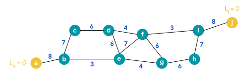
For the provided undirected weighted graph, assume the following:
- The number of iterations is 10.
- A number over an edge indicates its weight.
- The input provides seed labels \(L_a\) and \(L_j\) (for nodes \(a\) and \(j\)) with value 0; the input does not provide other seed labels.
Solution
This graph shows the final labels that the algorithm produces. The notation \(L_x\) denotes the label of node \(x\). The nodes are color-coded according to their labels.
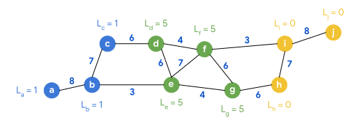
Note: the resulting labels depend on the order of node processing. This example assumes for simplicity that in each iteration the algorithm processes the active nodes in alphabetical order. In the actual implementation, this order is deterministic, but unspecified.
Algorithm details
This example assumes familiarity with the algorithm and the more detailed explanations in Example 1.
For the nodes that don't have input seed labels, the algorithm assigns a unique initial label for each node. Since the seed labels of nodes \(a\) and \(j\) already use 0, the algorithm uses 1, ..., 8 for the initial labels of the other nodes.
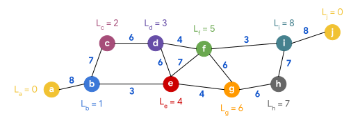
The algorithm marks all nodes as active for the first iteration.
Iteration #0: The algorithm processes the active nodes [\(a, b, c, d, e, f, g, h, i, j\)] in that order.
Here's the assignment of labels at the end of iteration #0:

- Nodes whose labels have changed: [\(a, c, d, e, g, h, i\)]
- Active nodes (neighbors of nodes with changed labels): [\(b, c, d, e, f, g, h, i, j\)]
Iteration #1: The algorithm processes the active nodes [\(b, c, d, e, f, g, h, i, j\)] in that order.
Here's the assignment of labels at the end of iteration #1:

- Nodes whose labels have changed: [\(d, h\)]
- Active nodes (neighbors of nodes with changed labels): [\(c, e, f, g, i\)]
Iteration #2: The algorithm processes the active nodes [\(c, e, f, g, i\)] in that order.
Here's the assignment of labels at the end of iteration #2:

- Nodes whose labels have changed: []
- Active nodes (neighbors of nodes with changed labels): []
As there are no active nodes, the algorithm stops.
External references
- The majority vote label propagation algorithm was introduced in Near Linear Time Algorithm to Detect Community Structures in Large-Scale Networks (Physical Review E, 2007).
- The largest-log-degree-first (LLF) heuristic for graph coloring used by the algorithm was introduced in Ordering Heuristics for Parallel Graph Coloring (Massive Graph Analytics, 2022).