Work with geospatial data in Bigtable

This page describes how to store and query geospatial data in Bigtable using the GoogleSQL geography functions. Geospatial data include geometrical representations of the Earth's surface in the form of points, lines, and polygons. You can group these entities into collections to track locations, routes, or other areas of interest.

Basic operations

The dedicated GoogleSQLgeography functions lets Bigtable optimize your database performance for geospatial calculations and query times. In the basic usage examples, we use a tourist_points_of_interest table with one column family called poi_data.

	poi_data
row key	name	location
p1	Eiffel Tower	POINT(2.2945 48.8584)

Write geography data

To write geospatial data to Bigtable columns, you need to provide string representations of geography entities in the GeoJSON or Well-Known Text (WKT) formats. Bigtable stores the underlying data as raw bytes, so you can provide any mix of entities in a single column (such as Points, LineStrings, Polygons, MultiPoints, MultiLineStrings, or MultiPolygons). The type of geospatial entity you provide is important at query time because you need to use the appropriate geography function to interpret the data.

For example, to add some attractions to the tourist_points_of_interest table, you can use the cbt CLI tool like so:

With WKT:

cbt set tourist_points_of_interest p2 poi_data:name='Louvre Museum'
cbt set tourist_points_of_interest p2 poi_data:location='POINT(2.3376 48.8611)'

cbt set tourist_points_of_interest p3 poi_data:name='Place Charles de Gaulle'
cbt set tourist_points_of_interest p3 poi_data:location='POLYGON(2.2941 48.8733, 2.2941 48.8742, 2.2957 48.8742, 2.2958 48.8732, 2.2941 48.8733)'

With GeoJSON:

cbt set tourist_points_of_interest p2 poi_data:name='Louvre Museum'
cbt set tourist_points_of_interest p2 poi_data:location='{"type": "Point", "coordinates": [2.3376, 48.8611]}'

cbt set tourist_points_of_interest p3 poi_data:name='Place Charles de Gaulle'
cbt set tourist_points_of_interest p3 poi_data:location='{"type": "Polygon", "coordinates": [[ [2.2941, 48.8733], [2.2941, 48.8742], [2.2957, 48.8742], [2.2958, 48.8732], [2.2941, 48.8733] ]] }'

Query geography data

You can query the tourist_points_of_interest table with GoogleSQL in Bigtable Studio and filter the results with geography functions. For example, to find all tourist attractions within 1500 meters of Trocadéro, you can use the ST_DWITHIN function:

SELECT _key, poi_data['name'], poi_data['location']
FROM points_of_interest
WHERE ST_DWITHIN(CAST(poi_data['location'] AS STRING), ST_GEOGPOINT(2.2874, 48.86322), 1500);

The result would be similar to the following:

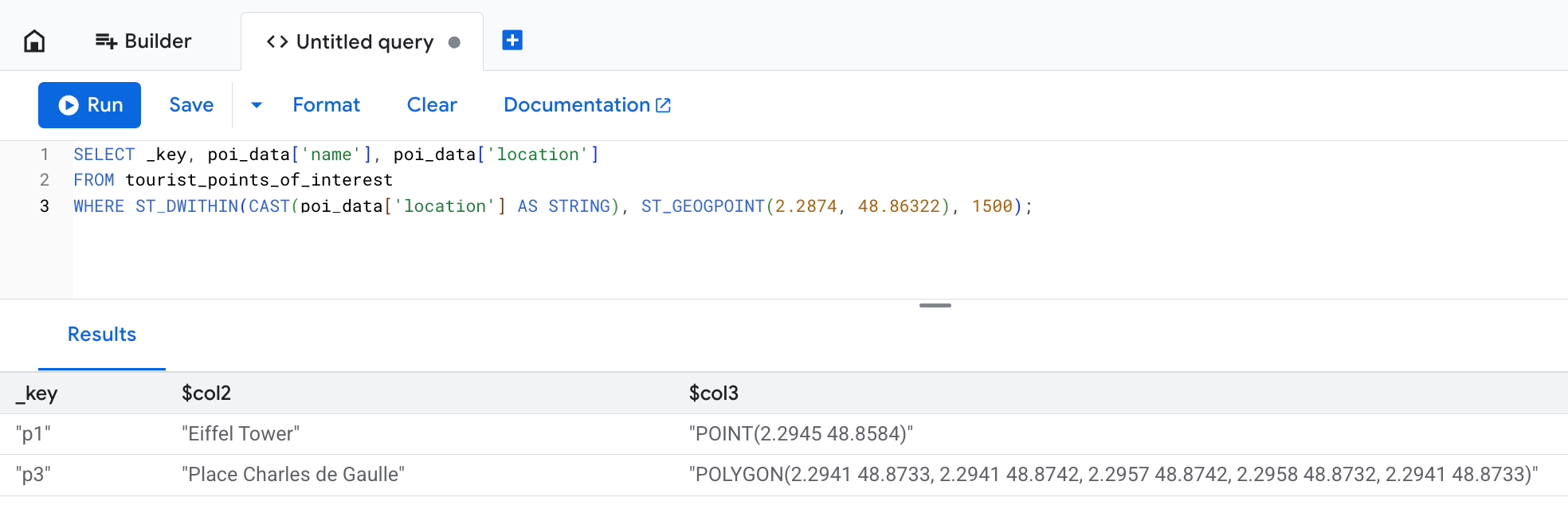
Screenshot showing the tourist_points_of_interest table in Bigtable Studio
with query results filtered with the ST_DWITHIN geography function.

The location column shows the original textual representation of the data provided in the write operation, but Bigtable stores it as bytes. In this example, even though Place Charles de Gaulle is defined as a polygon that stretches farther than the 1500 meter limit, it is included in the query results. That's because the ST_DWITHIN function returns true if any point contained in a geospatial entity is within the expected distance.

Advanced usage

The following sections describe how to use geography functions for complex scenarios like geofencing analysis. The Query optimization section explains how to use continuous materialized views for improved performance.

To illustrate advanced uses of geography functions in Bigtable, imagine a scenario where you are a researcher monitoring the behavior of emperor penguins who live on the southern side of the Snow Hill Island.

Your equipment provides hundreds of location pings for each penguin, so you create the penguin_movements table to store them:

	penguin_details
row key	penguin_id	timestamp	location
ping#123	pen_01	2025-12-06 08:15:22+00	POINT(-57.51 -64.42)
ping#124	pen_01	2025-12-06 10:22:05+00	POINT(-57.55 -64.43)
ping#125	pen_01	2025-12-07 12:35:45+00	POINT(-57.58 -64.41)
ping#126	pen_02	2025-12-12 06:05:11+00	POINT(-57.49 -64.39)

Example: Find who crossed the geofence

During the research, you observe penguin behavior around a specific feeding ground. Areas defined with virtual boundaries are commonly known as geofences. The feeding ground can be considered a geofenced area. You want to find out if any penguins visited the feeding ground on December 3, 2025. To answer the question, you use the ST_CONTAINS function, like so:

SELECT
  penguin_details['penguin_id'],
  penguin_details['location'],
  penguin_details['timestamp']
FROM
  penguin_movements
WHERE
  penguin_details['timestamp'] >= '2025-12-03 00:00:00 UTC'
  AND penguin_details['timestamp'] < '2025-12-04 00:00:00 UTC'
  -- The feeding ground boundary is defined with a WKT POLYGON entity
  -- Polygon's last point must be equal to its first point to close the loop
  AND ST_CONTAINS(
        ST_GEOGFROMTEXT('POLYGON((-57.21 -64.51, -57.23 -64.55, -57.08 -64.56, -57.06 -64.51, -57.21 -64.51))'),
        ST_GEOGFROMTEXT(CAST(penguin_details['location'] AS STRING))
      )

You get results similar to the following:

+------------+----------------------+------------------------+
| penguin_id |       location       |       timestamp        |
+------------+----------------------+------------------------+
| pen_01     | POINT(-57.15 -64.53) | 2025-12-03 08:15:22+00 |
| pen_02     | POINT(-57.18 -64.54) | 2025-12-03 14:30:05+00 |
| pen_10     | POINT(-57.10 -64.52) | 2025-12-03 11:45:10+00 |
+------------+----------------------+------------------------+

Example: Transform points to routes

To better visualize how the penguins travel, you decide to organize individual location pings into LineStrings by using the ST_MAKELINE function like so:

SELECT
  penguin_id,
  DATE(timestamp, 'UTC') AS route_date,
  ST_MAKELINE(ARRAY_AGG(location_cast_to_geog)) AS route
FROM (
  -- Sub-expression to sort all location pings by timestamp
  -- This way you make sure individual points can form a realistic route
  SELECT
    penguin_details['penguin_id'] AS penguin_id,
    -- Extract and cast timestamp once
    CAST(CAST(penguin_details['timestamp'] AS STRING) AS TIMESTAMP) AS timestamp,
    -- Extract and cast location once
    ST_GEOGFROMTEXT(CAST(penguin_details['location'] AS STRING)) AS location_cast_to_geog
  FROM
    penguin_movements
  ORDER BY
    -- Pre-sorts location pings for the ARRAY_AGG function
    penguin_id, timestamp ASC
)
GROUP BY
  penguin_id,
  route_date

With this query, you can get more advanced insights for your research. Expand the following sections to see example queries and results.

What is the daily travel distance for each penguin?

To calculate how much distance each penguin covers every day, you can use the ST_LENGTH function.

SELECT
  penguin_id,
  route_date,
  ST_LENGTH(route) AS daily_distance_meters
FROM (
  -- Subquery to aggregate points into daily routes
  SELECT
    penguin_id,
    DATE(timestamp, 'UTC') AS route_date,
    ST_MAKELINE(ARRAY_AGG(location_cast_to_geog)) AS route
  FROM (
    -- Sub-expression to sort all location pings by timestamp
    -- This way you make sure individual points can form a realistic route
    SELECT
      penguin_details['penguin_id'] AS penguin_id,
      -- Extract and cast timestamp once
      CAST(CAST(penguin_details['timestamp'] AS STRING) AS TIMESTAMP) AS timestamp,
      -- Extract and cast location once
      ST_GEOGFROMTEXT(CAST(penguin_details['location'] AS STRING)) AS location_cast_to_geog
    FROM
      penguin_movements
    ORDER BY
      -- Pre-sorts location pings for the ARRAY_AGG function
      penguin_id, timestamp ASC
  )
  GROUP BY
    penguin_id,
    route_date
) AS DailyRoutes;

This query returns a result similar to the following:

+------------+------------+-----------------------+
| penguin_id | route_date | daily_distance_meters |
+------------+------------+-----------------------+
| pen_01     | 2025-12-02 | 15420.7               |
| pen_03     | 2025-12-03 | 22105.1               |
| pen_32     | 2025-12-03 | 9850.3                |
+------------+------------+-----------------------+

How much of the daily route occurs within the geofenced area?

To answer this question, you filter the results with the ST_INTERSECTION function to check which parts of the penguin's route intersect with the geofenced area. Then, the ST_LENGTH function can help calculate the ratio of movement within the feeding grounds to the full distance traveled that day.

SELECT
  penguin_id,
  route_date,
  ST_LENGTH(ST_INTERSECTION(route, ST_GEOGFROMTEXT('POLYGON((-57.21 -64.51, -57.23 -64.55, -57.08 -64.56, -57.06 -64.51, -57.21 -64.51))'))) / ST_LENGTH(route) AS proportion_in_ground
FROM (
  -- Subquery to aggregate points into daily routes
  SELECT
    penguin_id,
    DATE(timestamp, 'UTC') AS route_date,
    ST_MAKELINE(ARRAY_AGG(location_cast_to_geog)) AS route
  FROM (
    -- Sub-expression to sort all location pings by timestamp
    -- This way you make sure individual points can form a realistic route
    SELECT
      penguin_details['penguin_id'] AS penguin_id,
      -- Extract and cast timestamp once
      CAST(CAST(penguin_details['timestamp'] AS STRING) AS TIMESTAMP) AS timestamp,
      -- Extract and cast location once
      ST_GEOGFROMTEXT(CAST(penguin_details['location'] AS STRING)) AS location_cast_to_geog
    FROM
      penguin_movements
    ORDER BY
      -- Pre-sorts location pings for the ARRAY_AGG function
      penguin_id, timestamp ASC
  )
  GROUP BY
    penguin_id,
    route_date
) AS DailyRoutes
WHERE
  ST_INTERSECTS(route, ST_GEOGFROMTEXT('POLYGON((-57.21 -64.51, -57.23 -64.55, -57.08 -64.56, -57.06 -64.51, -57.21 -64.51))'))

This query returns a result similar to the following:

+------------+------------+----------------------+
| penguin_id | route_date | proportion_in_ground |
+------------+------------+----------------------+
| pen_01     | 2025-12-03 | 0.652                |
| pen_03     | 2025-12-03 | 0.918                |
| pen_32     | 2025-12-04 | 0.231                |
+------------+------------+----------------------+

Optimize queries with continuous materialized views

Geospatial queries on large datasets can be slow because they might require scanning many rows. Bigtable doesn't support dedicated geospatial indexes, but you can improve your query performance with continuous materialized views.

To create a unique row key for such views, you can transform the GEOGRAPHY type into an S2 cell. S2 is a library that lets you perform complex trigonometry for sphere geometry. Calculating distances based on geographical coordinates can be computationally expensive. S2 cells can represent a specific area on the Earth's surface as a 64-bit integer, making them ideal for geospatial indexing with continuous materialized views.

To define an S2 cell, you call the S2_CELLIDFROMPOINT(location, level) function and provide the granularity level argument. This argument is a number between 0 and 30 and defines the size of each cell: the higher the number, the smaller the cell.

In the penguin research example, you can create a continuous materialized view indexed on each penguin's location and timestamp:

-- Query used to create the continuous materialized view
SELECT
  -- Create S2 cells for each penguin's location.
  -- Note that the `level` value is the same for each location so that
  -- every cell is the same size. This ensures consistency for your data.
  S2_CELLIDFROMPOINT(ST_GEOGFROMTEXT(CAST(penguin_details['location'] AS STRING)), level => 16) AS s2_cell_id,
  penguin_details['timestamp'] AS observation_time,
  penguin_details['penguin_id'] AS penguin_id,
  penguin_details['location'] AS location
FROM
  penguin_movements

Querying this view to answer the Who crossed the geofence? question becomes much more efficient with a two-phase approach. You first use the cell_id index in the continuous materialized view to quickly find candidate rows within the general vicinity, then apply the accurate ST_CONTAINS function on the reduced dataset:

SELECT
  idx.penguin_id,
  idx.location,
  idx.observation_time
FROM
  penguin_s2_time_index AS idx
WHERE
  -- Part one: use an approximate spatial filter and timestamp filter
  -- for fast scans on continuous materialized view keys.
  -- Use the S2_COVERINGCELLIDS function to create an array of S2 cells
  -- that cover the feeding ground polygon. The `level` argument must be the
  -- same value as the one you used to create the continuous materialized view.
  idx.s2_cell_id IN UNNEST(S2_COVERINGCELLIDS(
    ST_GEOGFROMTEXT('POLYGON((-57.21 -64.51, -57.23 -64.55, -57.08 -64.56, -57.06 -64.51, -57.21 -64.51))'),
    min_level => 16,
    max_level => 16,
    max_cells => 500
  ))
  AND idx.observation_time >= '2025-12-03 00:00:00 UTC'
  AND idx.observation_time < '2025-12-04 00:00:00 UTC'
  -- Part two: use ST_CONTAINS() on the returned set to ensure precision.
  -- S2 cells are squares, so they don't equal arbitrary geofence polygons.
  -- You still need to check if a specific point is contained within the area,
  -- but the filter applies to a smaller data set and is much faster.
  AND ST_CONTAINS(ST_GEOGFROMTEXT('POLYGON((-57.21 -64.51, -57.23 -64.55, -57.08 -64.56, -57.06 -64.51, -57.21 -64.51))'), idx.location);

Limitations

Bigtable doesn't support the following features when working with geography data:

Three-dimensional geometries. This includes the "Z" suffix in the WKT format, and the altitude coordinate in the GeoJSON format.
Linear reference systems. This includes the "M" suffix in WKT format.
WKT geometry objects other than geometry primitives or multipart geometries. In particular, Bigtable supports only Point, MultiPoint, LineString, MultiLineString, Polygon, MultiPolygon, and GeometryCollection.
ST_CLUSTERDBSCAN function isn't supported.

For constraints specific to GeoJson and WKT input formats, see ST_GEOGFROMGEOJSON and ST_GEOGFROMTEXT.

What's next?

Learn more about available geography functions. See GoogleSQL geography functions overview.