

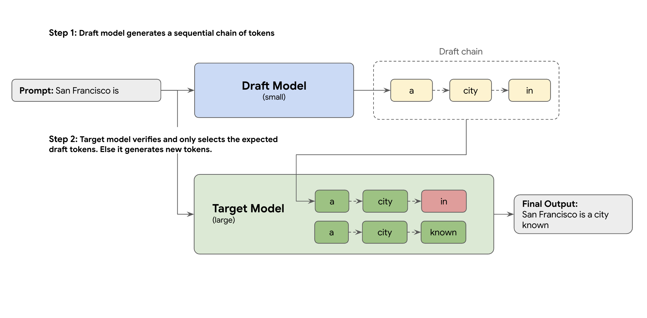
The solution is speculative decoding. This optimization technique speeds up the slow, sequential process of your large LLM (the target model) generating one token at a time, by introducing a draft mechanism.
This draft mechanism rapidly proposes several next tokens at once. The large target model then verifies these proposals in a single, parallel batch. It accepts the longest matching prefix from its own predictions and continues generation from that new point.
But not all draft mechanisms are created equal. The classic draft-target approach uses a separate, smaller LLM model as the drafter, which means you have to host, and manage more serving resources, causing additional costs.
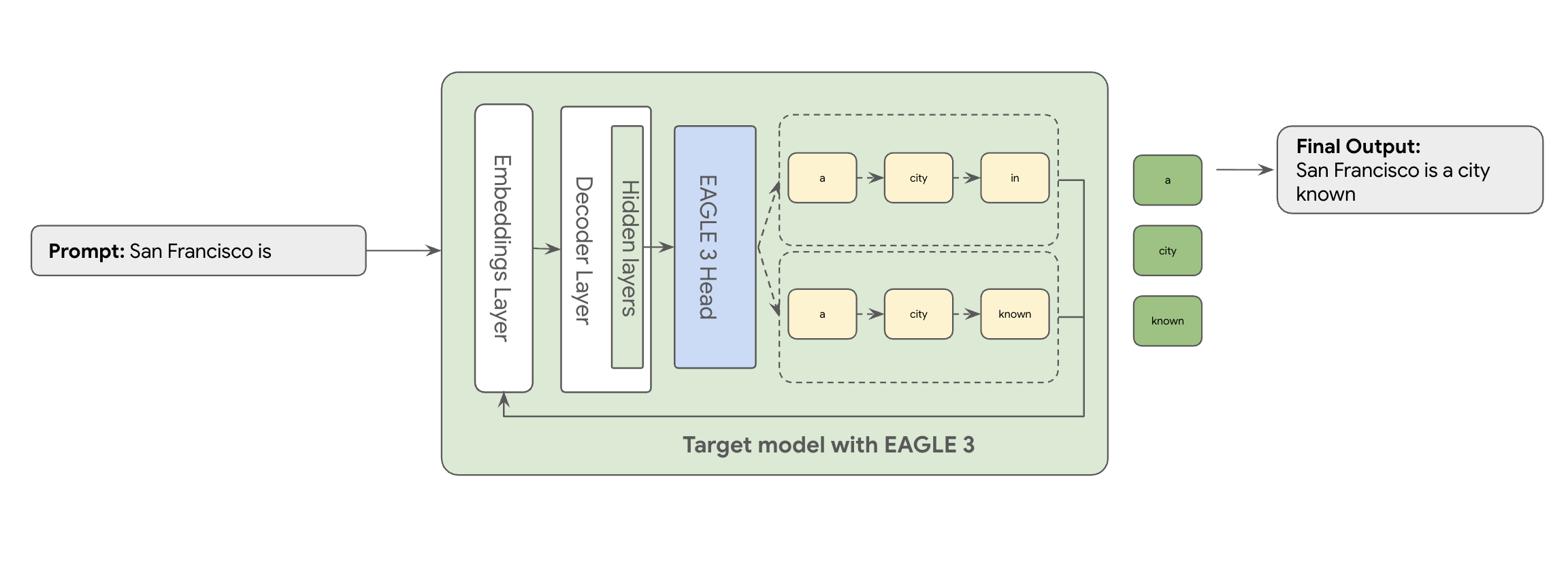
This is where EAGLE-3 (Extrapolative Attention Guided LEarning) comes in. EAGLE-3 is a more advanced approach. Instead of a whole separate model, it attaches an extremely lightweight 'draft head'—just 2-5% of the target model's size—directly to its internal layers. This head operates at both feature and token level, ingesting features from the target model's hidden states to extrapolate and predict a tree of future tokens.
The result? All the benefits of speculative decoding while eliminat[ing] the overhead of training and running a second model.
EAGLE-3's approach is far more efficient than the complex, resource-intensive task of training and maintaining a separate, multi-billion parameter draft model. You train only a lightweight 'draft head'—just 2% to 5% of the target model size—that is added as part to your existing model. This simpler, efficient training process delivers a significant 2x-3x decoding performance gain for models like Llama 70B (depending on the workload types, e.g., multi-turn, code, long context and more).
But moving even this streamlined EAGLE-3 approach from a paper to a scaled, production-ready cloud service is a real engineering journey. This post shares our technical pipeline, key challenges, and the hard-won lessons we learned along the way.
Challenge #1: Preparing the data
The EAGLE-3 head needs to be trained. The obvious first step is to grab a generic public available dataset. Most of these datasets present challenges, including:
- Strict Terms of Use: These datasets are generated using models that do not allow using them to develop models that would compete with original providers.
- PII Contamination: Some of these datasets contain significant PII, including names, locations, and even financial identifiers.
- No quality guaranteed: Some datasets only work great for general "demo" use cases, but not work best for real customers' specialized workload.
Using this data as-is is not an option.
Lesson 1: Build a Synthetic Data Generation Pipeline
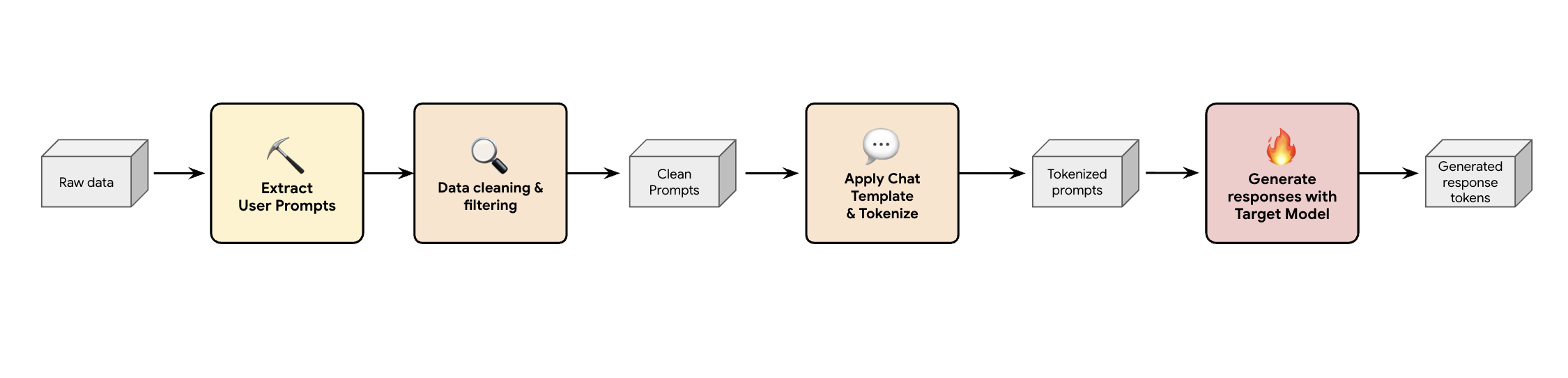
One solution is to build a synthetic data generation pipeline. Depending on our customer's use cases, we select the right dataset not only with good-quality but also matches best with our customer's production traffic for various different workloads. Then you can extract only the user prompts from these datasets and apply rigorous DLP (Data Loss Prevention) and PII filtering. These clean prompts apply a chat template, tokenize them and then they can be fed into your target model (e.g., Llama 3.3 70B) to collect its responses.
This approach provides target-generated data that is not only compliant and clean, but also well-matched to the model's actual output distribution. This is ideal for training the draft head.
Challenge #2: Engineering the training pipeline
Another key decision is how to feed the EAGLE-3 head its training data. You have two distinct paths: online training, where embeddings are 'generated on the fly', and offline training, where 'embeddings are generated before training'.
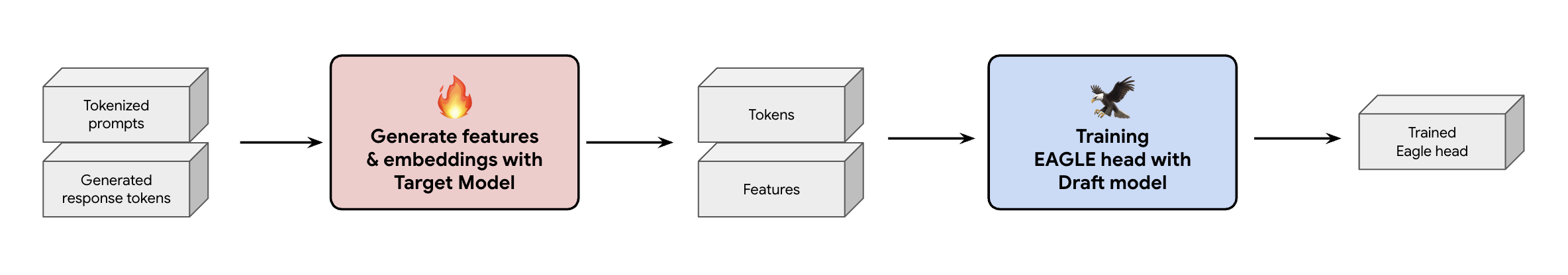
In our case, we chose an offline training approach because it requires much less hardware than online training. This process involves pre-calculating all the features and embeddings before we train the EAGLE-3 head. We save them to GCS and they become the training data for our lightweight EAGLE-3 head. Once you have the data, the training itself is fast. Given the diminutive size of the EAGLE-3 head, initial training with our original dataset required approximately one day on a single host. However, as we've scaled our dataset, training times have commensurately increased, now spanning several days.
This process taught us two not negligible lessons you need to keep in mind.
Lesson 2: Chat Templates Are Not Optional
While we were training for the instruction-tuned model, we found that EAGLE-3 performance can vary a lot when the chat template is not right. You must apply the target model's specific chat template (e.g., Llama 3's) before you generate the features and embeddings. If you just concatenate raw text, the embeddings will be incorrect, and your head will learn to predict the wrong distribution.
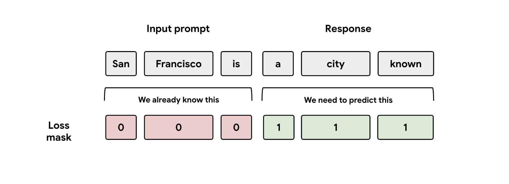
Lesson 3: Mind the Mask
During training, the model is fed both the prompt and response representations. But the EAGLE-3 head should only be learning to predict the response representation. You must manually mask the prompt part in your loss function. If you don't, the head wastes capacity learning to predict the prompt it was already given, and performance will suffer.
Challenge #3: Serving and Scaling
With a trained EAGLE-3 head, we proceeded to the serving phase. This phase introduced significant scaling challenges. Here are our key learnings.
Lesson 4: Your Serving Framework Is Key
By working closely in partnership with the SGLang team, we successfully landed EAGLE-3 to production with best performance. The technical reason is that SGLang implements a crucial tree attention kernel. This special kernel is crucial because EAGLE-3 generates a 'draft tree' of possibilities (not just a simple chain), and SGLang's kernel is specifically designed to verify all of those branching paths in parallel in a single step. Without this, you're leaving performance on the table.
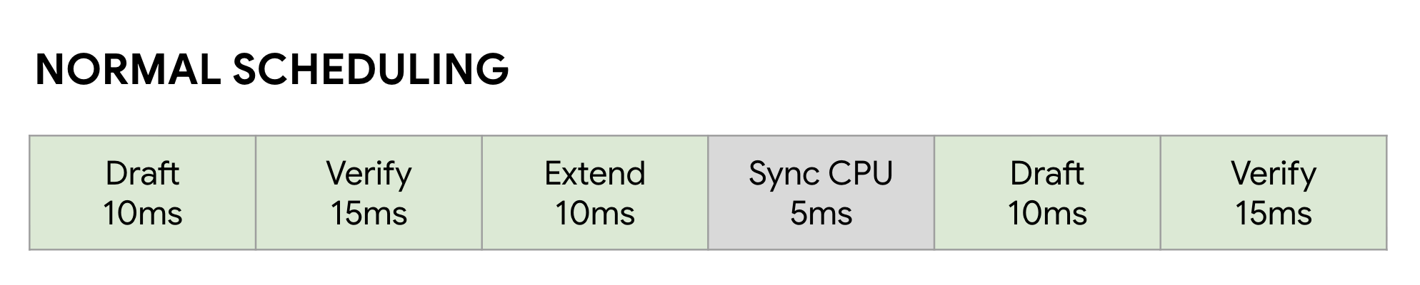
Lesson 5: Don't Let your CPU Bottleneck your GPU
Even after accelerating your LLM with EAGLE-3, you can hit another performance wall: the CPU. When your GPUs are running LLM inference, unoptimized software will waste a huge amount of time on CPU overhead—such as kernel launch and metadata bookkeeping. In a normal synchronous scheduler, the GPU runs a step (like Draft), then idles while the CPU does its bookkeeping and launches the next Verify step. These sync bubbles add up, wasting huge amounts of valuable GPU time.
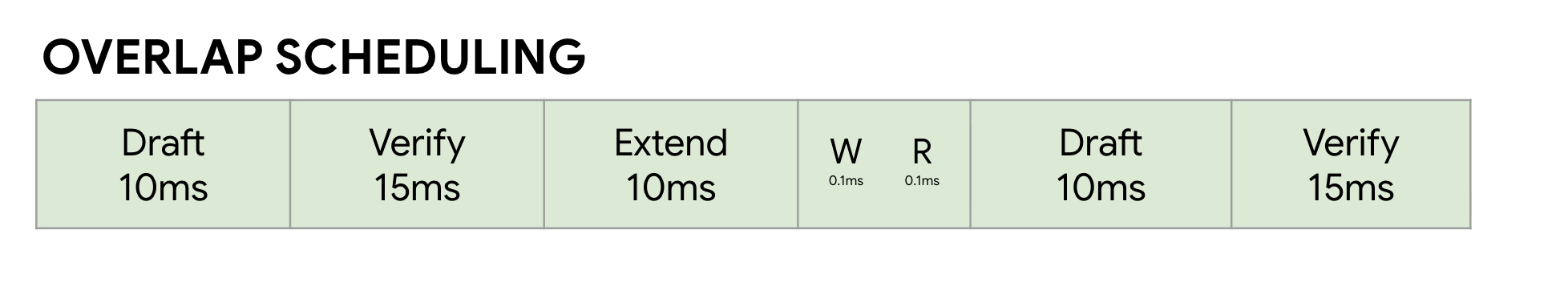
We solved this by using SGLang's Zero-Overhead Overlap Scheduler. This
scheduler is specifically tuned for speculative decoding's multi-step Draft ->
Verify -> Draft Extend workflow . The key is to overlap computation. While the
GPU is busy running the current Verify step, the CPU is already working in
parallel to launch the kernels for the next Draft and Draft Extend steps .
This eliminates the idle bubble by ensuring the GPU's next job is always ready,
using a FutureMap, a smart data structure that lets the CPU prepare the next
batch WHILE the GPU is still working.
By eliminating this CPU overhead, the overlap scheduler gives us an additional 10% - 20% speedup across the board. It proves that a great model is only half the battle; you need a runtime that can keep up.
Benchmark Results
After this journey, was it worth it? Absolutely.
We benchmarked our trained EAGLE-3 head against the non-speculative baseline using SGLang with Llama 4 Scout 17B Instruct. Our benchmarks show a 2x-3x speedup in decoding latency and significant throughput gains depending on the workload types.
See the full details and benchmark it yourself using our comprehensive notebook.
Metric 1: Median Time Per Output Token (TPOT)
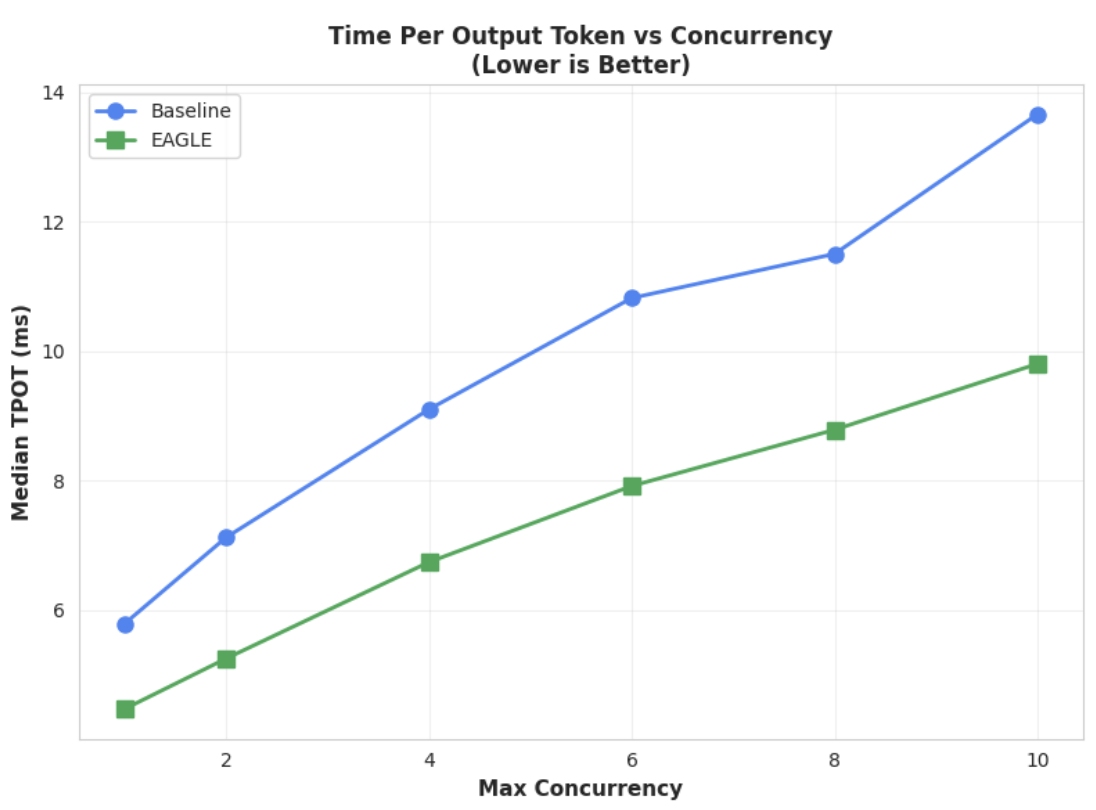
This chart shows the better latency performance of EAGLE-3. The Time Per Output Token (TPOT) chart shows EAGLE-3-accelerated model (green line) consistently achieves a lower (faster) latency than the baseline (blue line) across all tested concurrency levels.
Metric 2: Output Throughput
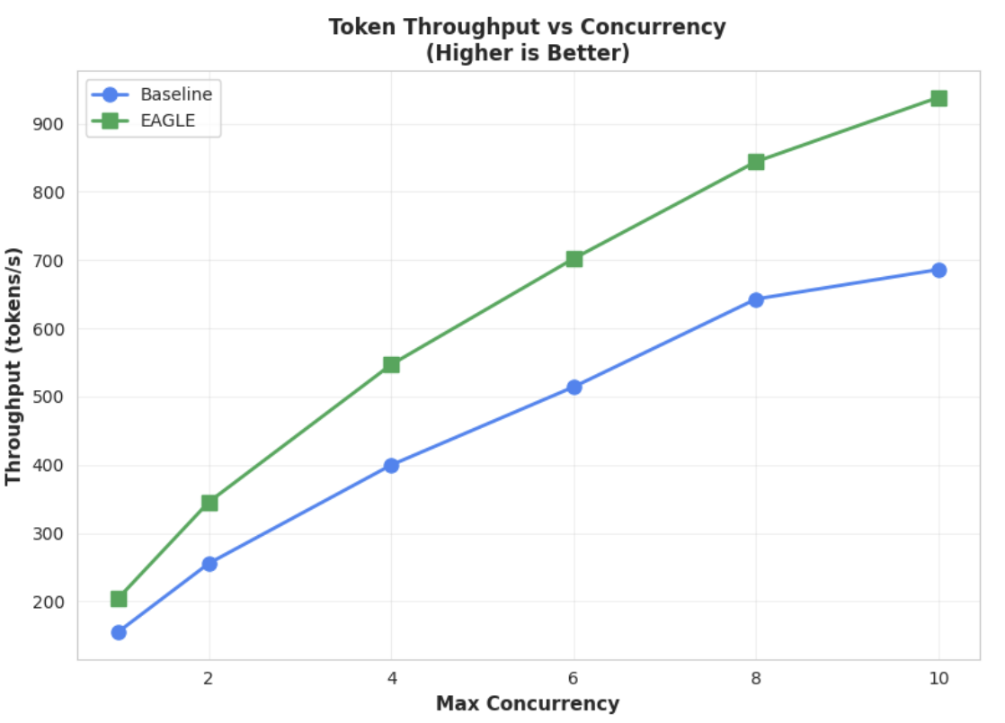
This chart further highlights EAGLE-3's throughput advantage. The Token Throughput vs. Concurrency chart clearly demonstrates that the EAGLE-3-accelerated model (green line) consistently and substantially outperforms the baseline model (blue line).
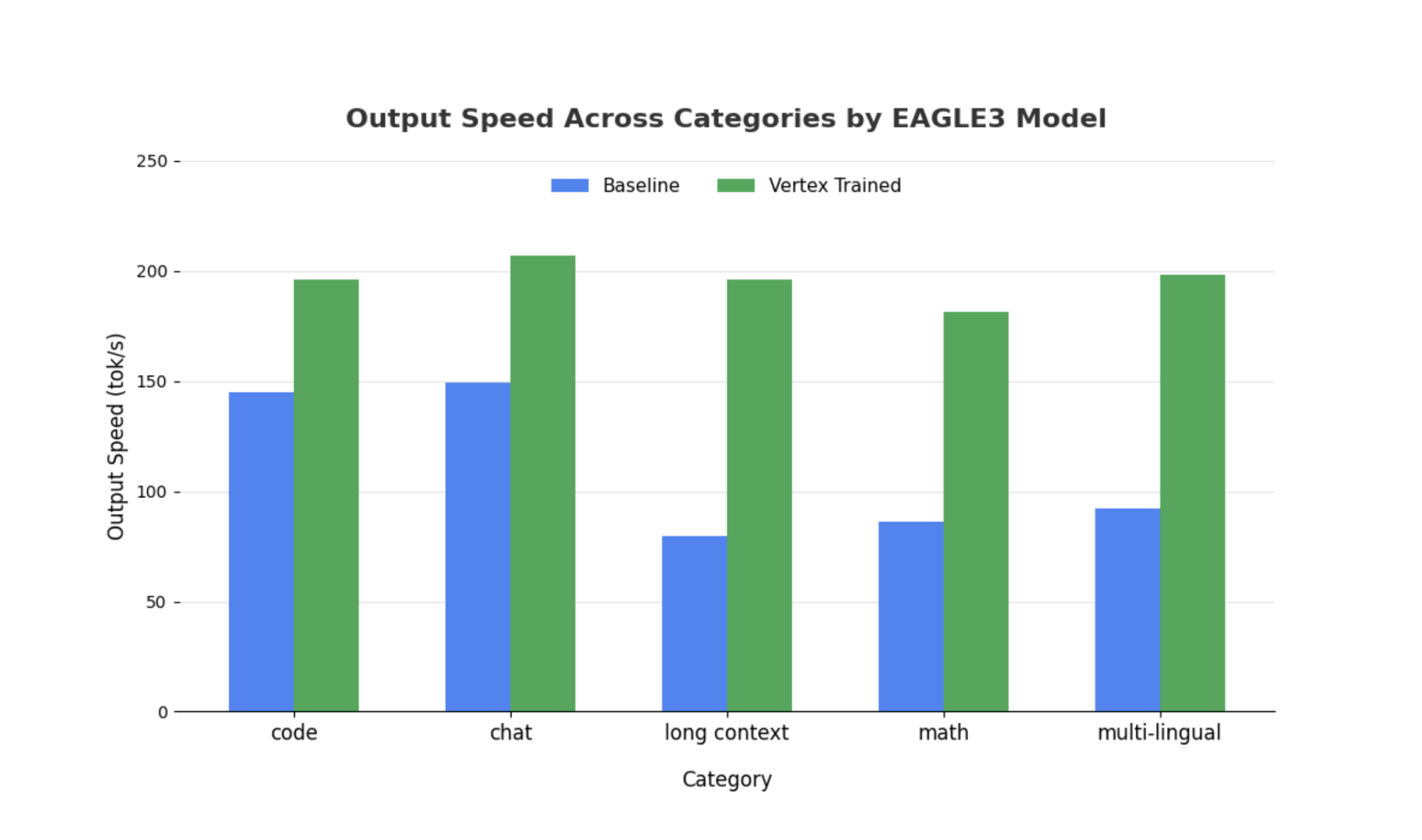
While similar observations hold true for larger models, it is worth noting that an increase in Time to First Token (TTFT) may be observed compared to other performance metrics. Also, these performances vary according to the task task-dependent, as illustrated by the following examples:
Conclusion: Now It's Your Turn
EAGLE-3 isn't just a research concept; it's a production-ready pattern that can deliver a tangible 2x speedup in decoding latency. But getting it to scale requires a real engineering effort. To reliably deploy this technology for your users, you must:
- Build a compliant synthetic data pipeline.
- Correctly handle chat templates and loss masks and train the model on a large scale of dataset.
On Vertex AI, we've already streamlined this entire process for you, providing an optimized container and infrastructure designed to scale your LLM-based applications. To get started, check out the following resources:
Thanks for reading
We welcome your feedback and questions about Vertex AI.
Acknowledgements
We would like to express our sincere gratitude to the SGLang team—specifically Ying Sheng, Lianmin Zheng, Yineng Zhang, Xinyuan Tong, Liangsheng Yin as well as SGLang/SpecForge team —specifically Shenggui Li, Yikai Zhu—for their invaluable support throughout this project. Their generous assistance and deep technical insights were instrumental to the success of this project.