Chart and dashboard controls in Cloud Monitoring let you inspect
time-series data by highlighting specific lines, pinning a reference time,
zooming into time or value ranges, and toggling auto-refresh. When
troubleshooting, you can also configure charts to display only outliers,
overlay past data for comparison, or correlate metrics with logs and trace
exemplars.
These controls are available on charts in custom dashboards, in
[Metrics Explorer](https://docs.cloud.google.com/monitoring/charts/metrics-explorer), and when configuring alerting
conditions. To add charts to a dashboard, see [Display metric data on a custom
dashboard](https://docs.cloud.google.com/monitoring/charts). To isolate spikes or trends by label key in
Metrics Explorer, see [Break down a chart by labels](https://docs.cloud.google.com/monitoring/charts/breakdown-chart-by-labels).
## Highlight time series
You can examine individual time series by manipulating either the chart or
its legend. This section describes how you can change the chart
display so that one or more time series are highlighted while all other time
series are dimmed.
### Highlight a single time series
To highlight a single time series, do one of the following:
- Place your pointer on the graph line at a specific point in time. As you move your pointer on the graph, each time it touches a graph line, that line is highlighted.
- Click the checkbox in the corresponding row of the table legend or
click the line in the graph. After you select a specific line, you can
move your pointer without the selection changing.
- To highlight a different line in the graph, select it.
- To remove the highlight for a line, click in an unused area of the graph or expand the legend and then clear that line's checkbox.
For example, in the following screenshot, the `halyard` time series has been
selected:

### Highlight multiple time series
To highlight all lines between `line-N` and `line-O`,
select `line-N`, press `Shift`, and then select `line-O`.
To highlight multiple lines, do one of the following:
- Press `Control` or `Command`, and then select the lines of interest from the graph.
- In the legend, select the checkboxes for the lines of interest.
To remove the highlight on a time series, select its row in the legend.
To remove all highlights, click in an unused area of the graph.
## Set a reference time
To select a reference time on a graph, you set a *pin* at the reference time.
An unset pin appears on the graph when you place your pointer on the numbers
along the *X*-axis. The unset pin is a dim line with an oval at its
base that displays a time and a pin symbol.
When you set a pin, the following events occur:
- A blue line with an oval at its base appears on the graph. The base displays the reference time and a **Dismiss** button. To remove the pin, click **Dismiss**.
- The legend field **Value** displays the value of the time series at the reference time.
- When the chart is on a dashboard, a pin is set on every chart on the dashboard.
You can only set one pin on a chart, and you can either set the pin at the
current time or at a specific time:
- To set the pin at the current time, click **Value** in the legend heading
of the chart.
- To set the pin at a specific time, place your pointer along the *X*-axis
at that time, and then click the oval.
For example, the following screenshot illustrates a chart with a pin at
3:30 PM and a pointer at time 3:42 PM. The tooltip displays the
timestamp that corresponds to the pointer position. The tooltip displays 440ms,
which is the value of the time series `server_latency` at 3:42 PM.
The legend displays 1.505ms, which is the value of the time series
`server_latency` at 3:30 PM:

## Change the graph resolution
There are multiple ways that you can change the resolution of a chart.
For information about how to change the resolution of all charts on a dashboard,
see [Set the display period](https://docs.cloud.google.com/monitoring/charts/working-with-charts#display-period).
### Expand a specific time interval
To magnify the graph in a specific time interval, do the following:
1. Place your pointer in the graph area at one end of the time interval that you want to view in more detail.
2. Drag your pointer horizontally to the other end of the interval. The drag
action creates a dim region between two time selectors.
After you release the pointer button, the graph is redrawn using the range
of *X* -axis values that you selected. The *Y*-axis range is automatically
adjusted based on the values in the time period you selected.
3. Optional: Change the vertical resolution of the chart.
When you select a time period for any chart on a dashboard, the dashboard
disables auto-refresh and indicates that behavior by showing the
button on the dashboard toolbar.
To enable auto-refresh, click the button.
### Expand the time resolution around a point in time
To magnify the graph around a specific point in time, do the following:
1. Place your pointer in the graph area at the point in time that you want to view in more detail.
2. To expand or contract the time axis, press `Control` or `Command`, and then use two fingers on a trackpad pointer or the scroll wheel on a pointer.
If a chart sets a time-range override, then you can't change the chart's
resolution by using your pointer.
### Shift the time range
To shift the range of times being displayed, do the following:
1. Place your pointer in the graph area at the point in the time interval that you want to view in more detail.
2. To display earlier or later data, press `Control` or `Command` and then select and drag your pointer.
### Expand the vertical resolution
To magnify an interval of values, follow these steps:
1. Place your pointer in the graph area at one end of the value range that you want to view in more detail.
2. Drag your pointer vertically to the other end of the range. The
drag action creates a dim region between two values on the *Y*-axis.
After you release the pointer button, the graph is redrawn using the
*Y*-axis range that you selected.
3. Optional: Change the horizontal resolution of the chart.
When you select a time period for any chart on a dashboard, the dashboard
disables auto-refresh and indicates that behavior by showing the
button on the dashboard toolbar.
To enable auto-refresh, click the button.
### Reset the resolution
To reset a chart's zoom level, do one of the following:
- To reset an individual chart, click **Reset zoom** on the chart's toolbar.
- To reset all charts on a dashboard to the global dashboard display period, click **Reset zoom** on the dashboard toolbar.
Resetting the zoom level for a dashboard doesn't affect charts that set a
time-range override. For those charts, you can't change the chart's
resolution by using your pointer.
### Set the display period or time range
A chart can display data for periods ranging from one hour to six weeks. The
system determines the display period for a chart as follows:
- If the chart's **Time range override** field is configured, then the
system uses the specified time range. This field lets you enter a
relative or an absolute time range.
- If the chart's **Time range override** field isn't configured, then the
system uses the time-range setting of its parent, which is either
Metrics Explorer or a custom dashboard.
Configure a chart's time-range override when you want that chart to show data
over a longer or shorter time range than is appropriate for other dashboard
widgets.
Changing the time range on a chart can result in realignment of the time series.
For conceptual information, see
[Alignment: within-series regularization](https://docs.cloud.google.com/monitoring/api/v3/aggregation#alignment-intro).
For a new project, data may not be available for all parts of the range.
## Select dynamic or static data
Charts display data within a window of time. By default, this window advances,
with "now" always at the right edge of the chart. The time
selection determines the window into the past, for example, one
hour. The data on the chart is dynamic; as new data is generated, it appears
at "now". By default, this
behavior is enabled.
You can keep the time window from changing by turning off auto-refresh.
This static option is useful when you want to study a past event. If you turn
off **Auto-Refresh** , the button turns dim and is labeled **OFF**.
Dashboards provide a single **Auto-Refresh** button that controls automatic
data updates:
- Relative time ranges, such as **Last 1 hour**, automatically advance when auto-refresh is enabled.
- Absolute time periods, such as a specific date range, don't advance. The auto-refresh setting is ignored.
When building a chart on the **Metrics Explorer** page, auto-refresh is
always on.
## Show outliers
Sorting the time series that match a query, and then limiting the number of
time series that are charted, lets you chart the anomalous lines
rather than the highly representative ones. Limiting the number of lines charted
also helps verify that individual charts are both responsive and
intelligible. You can limit the number of time series that are displayed when
you display data by using line, stacked bar, stacked area, and heatmap widgets.
> [!IMPORTANT]
> **Key Point:** Sorting the time-series data and then limiting the number of charted time series reduces visual noise when visualizing large datasets, which can mean faster diagnosis of system problems. Limiting the amount of data that is charted also yields better chart performance.
For example, the following screenshot illustrates a chart in color mode.

This chart contains many lines and is difficult to interpret. To restrict
the chart to only show the top three lines, ranked by mean, use the
**Sort \& Limit** fields.
A small annotation on the chart describes the display criteria. In the
background, shown in gray, is an outline of all time-series data. You cannot
disable the gray content.

### Charts on dashboards
To configure a chart to display the top or bottom outliers,
do the following:
1. In the Google Cloud console, go to the **Dashboards** page:
[Go to **Dashboards**](https://console.cloud.google.com/monitoring/dashboards)
If you use the search bar to find this page, then select the result whose subheading is
**Monitoring**.
2. In the toolbar of the Google Cloud console, select your Google Cloud project. For [App Hub](https://docs.cloud.google.com/app-hub/docs/overview) configurations, select the App Hub host project or management project.
3. Select a dashboard.
4. In the chart's toolbar,
select **Edit**.
5. In the chart's **Query** pane, go to the **Sort \& limit** element, and
then complete the dialog. The options let you select how time series
are ranked and whether you want the top or bottom outliers to be
shown.
If the **Sort \& limit** element isn't shown, then click
**Add query element**.
### Metrics Explorer
To configure a chart to display the top or bottom outliers,
do the following:
1. In the Google Cloud console, go to the
**Metrics explorer** page:
[Go to **Metrics explorer**](https://console.cloud.google.com/monitoring/metrics-explorer)
If you use the search bar to find this page, then select the result whose subheading is
**Monitoring**.
2. In the toolbar of the Google Cloud console, select your Google Cloud project. For [App Hub](https://docs.cloud.google.com/app-hub/docs/overview) configurations, select the App Hub host project or management project.
3. Select a resource type and metric type to chart.
4. In the chart's **Query** pane, go to the **Sort \& limit** element, and
then complete the dialog. The options let you select how time series
are ranked and whether you want the top or bottom outliers to be
shown.
If the **Sort \& limit** element isn't shown, then click
**Add query element**.
## Compare current to past data
The **Compare to Past** option lets you select a time range from the past
by specifying the hours, days, or weeks. The data from that time
range is then superimposed as a dotted line over the current data on a line
chart. The legend also shows past and present values.
**Compare to Past** is available only for line charts.
The data superimposed on your chart is for the same
[display period](https://docs.cloud.google.com/monitoring/charts/working-with-charts#display-period) as your chart but from the specified time
in the past. For example, consider a chart that shows data from
10 am to 11 am. If you specify data from the previous 2 weeks as 'past data',
then you see data collected between 10 am and 11 am and from the previous
2 weeks.
If there is no data available from the requested period, then there aren't any
changes on the chart.
The following screenshots show the same chart with and without the
data from 2 weeks ago.
**Without past data:**

**With past data** and one time series highlighted:

### Charts on dashboards
To compare current to past data on a chart, do the following:
1. In the Google Cloud console, go to the **Dashboards** page:
[Go to **Dashboards**](https://console.cloud.google.com/monitoring/dashboards)
If you use the search bar to find this page, then select the result whose subheading is
**Monitoring**.
2. In the toolbar of the Google Cloud console, select your Google Cloud project. For [App Hub](https://docs.cloud.google.com/app-hub/docs/overview) configurations, select the App Hub host project or management project.
3. Select a dashboard.
4. In the chart's toolbar,
select **Edit**.
5. In the **Display** pane, click the **Compare to Past** option.
6. Set the **Value** and **Scope** fields to specify how far in the past
to go.
For example, if **Value** is `2` and **Scope** is `weeks`, then the chart
displays the current data and data from 2 weeks in the past.
### Metrics Explorer
To compare current to past data on a chart, do the following:
1. In the Google Cloud console, go to the
**Metrics explorer** page:
[Go to **Metrics explorer**](https://console.cloud.google.com/monitoring/metrics-explorer)
If you use the search bar to find this page, then select the result whose subheading is
**Monitoring**.
2. In the toolbar of the Google Cloud console, select your Google Cloud project. For [App Hub](https://docs.cloud.google.com/app-hub/docs/overview) configurations, select the App Hub host project or management project.
3. Select a resource type and metric type to chart.
4. In the chart's **Display** pane, expand
**Compare to past** ,
select **Enable compare to past** , and then enter a value for the
**Timeshift duration**.
For example, if the **Timeshift duration** field is set to **1w** and
the time-range selector is set to **Last 1 hour**, then the chart
displays one hour of current data and one hour of data from
one week in the past.
## Configure heatmap chart options
Heatmap charts display distribution-valued metrics. This section describes how
you can modify the displays of these charts to show percentiles and exemplars.
Exemplars are a way to associate arbitrary data with metric data. You can use
them to attach non-metric data to measurements.
One use of exemplars is to associate trace data with metric data.
When Monitoring displays the metric data, the chart is
annotated when an exemplar exists. These annotations let you correlate
your metric and trace data. For more information, see
[Correlate metrics and traces by using exemplars](https://docs.cloud.google.com/stackdriver/docs/instrumentation/advanced-topics/exemplars).
### Show percentile lines on a heatmap chart
To hide or show the overlay of the 50th, 95th, and 99th percentile lines
on a heatmap chart, click  **Percentile lines**
in the chart toolbar. By default, the percentile lines are shown.
The following screenshot illustrates the chart with the percentile
lines displayed:

### Show only percentile lines on a heatmap chart
To hide or show the heatmap chart, click  **Heatmap**
in the chart toolbar.
The following screenshot shows the chart when the percentile lines are
shown, but the heatmap itself has been hidden:

### Show exemplars on a heatmap chart
For heatmap charts on dashboards,
to hide or show Cloud Trace exemplars,
click  **Trace exemplars** in the chart toolbar.
Exemplars aren't always available.
The following screenshot illustrates a section of a heatmap, where each
light-blue circle corresponds to a trace exemplar:

The previous heatmap was generated by running a
[Java instrumentation sample](https://docs.cloud.google.com/stackdriver/docs/instrumentation/setup/java).
This sample uses OpenTelemetry, an open-source tracing package, to instrument
a Java application.
To view the details of a specific exemplar, select it. The displayed details
include a graph that shows the trace spans. For more information, see
[Find and explore traces](https://docs.cloud.google.com/trace/docs/finding-traces).
## Correlate metric and log data
Correlating metric and log data is available only for charts on dashboards.
This feature isn't available if you use Metrics Explorer.
When you view a chart, you might want to explore log data that was
written against the same resource as the charted metric data. For example, if
you see a spike or a dip in a chart, then you might want to explore log entries
so that you can get additional information about the system.
One way you can correlate your metric and log data, is to use chart options to
open a flyout that displays both the chart and selected log entries. You can
then use the toolbars and menus in the flyout to explore your metric and
log data. For example, you might add filters to the metric query, modify the
logging query, or expand and explore log entries.
The following screenshot illustrates the flyout:
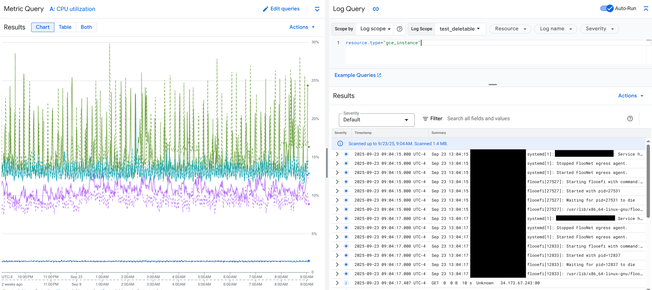
The flyout doesn't display all log entries that match the dashboard's
time-range selector. Instead, the system creates a logging query that is based
on the metric query. The logging query includes any applicable
[variables](https://docs.cloud.google.com/monitoring/dashboards/filter-permanent), but it doesn't include
dashboard-level filters.
#### View metric and log data
You can correlate metric and log data when a chart displays any metric type
except a log-based metric or a Prometheus metric. When a chart displays
a log-based metric, a Prometheus metric, or when it doesn't display metric data,
you can't correlate metric and log data.
To open the flyout that displays both metric and log data, do one of the
following:
- To filter log data only by the resource type and applicable variables,
in the chart's toolbar, click **More chart options** ,
and then select **Inspect related logs**.
- To show log entries that correlate with a specific time series,
in the chart, use your pointer to select a point on the time series,
and then go to the tooltip and
select **Inspect related logs**.
In this mode, the flyout modifies the time-range selector to be five minutes
before and after the timestamp of the selected point.
If your chart doesn't display an **Inspect related logs** option, then it
doesn't support metric and log correlation.
#### Save your changes
You can save the chart or logs panel shown in the flyout, including any
changes that you make, to a custom dashboard. If you save the chart to the
same dashboard from which you opened the flyout, then a new chart is created
on the dashboard.
To save the chart or logs panel to a custom dashboard, open the
widget's **Actions** menu, select **Save to dashboard**, and then complete
the dialog. You can select an existing custom dashboard or you can create
a dashboard and then save the widget.
#### Close the flyout
To close the flyout, in the toolbar, click **Cancel**.
## Show the chart configuration
### Charts on dashboards
To view the configuration of a chart displayed on a dashboard, click
**Query stats**:

The previous example lists the metric type that is charted, the filters,
the grouping options, and the alignment options.
### Metrics Explorer
The chart configuration fields are always visible.
## Show the chart legend
### Charts on dashboards
You can show or hide the legends of all charts on a dashboard or of each
chart individually:
- To show or hide the legends of every chart in a dashboard, in the dashboard toolbar, click **Settings** and then select **Condensed** or **Table**.
- To show or hide the legend of a particular chart, click **Expand legend** , or select **Expand chart legend** in the **More chart options** menu.
### Metrics Explorer
- To show a chart's full legend, in the toggle labeled **Chart Table Both** , select **Both**.
- To hide a chart's full legend, in the toggle labeled **Chart Table Both** , select **Chart**.
For more information, see [Show and hide legends](https://docs.cloud.google.com/monitoring/charts/working-with-legends#toggling-legends).
## What's next
- To filter widgets on a dashboard, do the following:
- [Add temporary filters](https://docs.cloud.google.com/monitoring/charts/filter-dashboard).
- [Add permanent filters](https://docs.cloud.google.com/monitoring/dashboards/filter-permanent).
- To configure the visual display of a chart by using the
Google Cloud console, see [Set chart display options](https://docs.cloud.google.com/monitoring/charts/chart-view-options).
- To configure the chart legends by using the
Google Cloud console, see [Configure legends](https://docs.cloud.google.com/monitoring/charts/working-with-legends).
- For an introduction to Cloud Monitoring metrics, see
[Metrics, time series, and resources](https://docs.cloud.google.com/monitoring/api/v3/metrics).
- To create your own metrics, see [User-defined metrics](https://docs.cloud.google.com/monitoring/custom-metrics)
and [Log-based metrics](https://docs.cloud.google.com/logging/docs/view/logs_based_metrics).