Selecting metrics and aggregation options in Metrics Explorer lets you
focus on the exact numeric time-series data collected by your Google Cloud project
that you want to analyze. When building a temporary chart, you can choose a
metric type and apply filters, grouping, and alignment by using menus or by
writing a query.
## Select the data to display
To configure which time series to display on a chart, you can
build a query by making selections from menus, or you can write a query.
When you write a query, you select your query language and then you use a
query editor or a text-based interface:
- [Prometheus Query Language (PromQL)](https://docs.cloud.google.com/monitoring/promql) queries specify time series
and how those time series are grouped and aligned.
The PromQL interface supports an editor with suggestions.
It isn't generally possible to convert PromQL queries into forms
that can be used by the other interfaces. Your unsaved queries are
discarded when you switch to or from the PromQL tab.
- [Monitoring filter](https://docs.cloud.google.com/monitoring/api/v3/filters) queries
specify the time series but don't include grouping or alignment statements.
Any time series that Monitoring can chart can be specified
by using a Monitoring filter. For example, to chart the number
of processes running on a VM, you must use a
Monitoring filter that specifies a function.
It isn't always possible to convert a Monitoring filter
into the form required by other interfaces. Therefore, your query might
be discarded if you switch to a different interface.
Queries typically specify a metric type, a resource type, and filters:
- A *metric type* identifies the measurements to be collected from a
resource. It includes a description of what is being measured
and how the measurements are interpreted. A *metric type* is sometimes
referred to as a *metric* . An example of a metric is "CPU utilization".
For conceptual information, see
[Metric types](https://docs.cloud.google.com/monitoring/api/v3/metric-model#metric_types).
- A *resource type* specifies from which resource the metric data is
captured. *Resource type* is sometimes called the
*monitored resource type* or the *resource* . An example of a
resource is a "Compute Engine virtual machine (VM) instance".
For conceptual information, see
[Monitored resources](https://docs.cloud.google.com/monitoring/api/v3/metric-model#resource-overview).
- A *filter* lets you remove data from the query result that doesn't
match some criterion, like a resource type or the value of a label.
We recommend filtering on the labels defined on
[monitored-resource types](https://docs.cloud.google.com/monitoring/api/resources) instead
of labels defined on [metric types](https://docs.cloud.google.com/monitoring/api/metrics)
when possible, particularly if you are querying high-cardinality metrics.
If you have a resource label and a metric label that capture
similar information, then use the resource label in your queries.
For example, if your monitored resource includes a `cluster`
label and your metric includes a `kubernetes_cluster_name` label that
captures similar information, then filter on the resource `cluster`
label.
PromQL queries include grouping and alignment statements. However, when you
write a Monitoring filter or use
menus to select the time series to chart, you configure the grouping and
alignment settings by using menus.
> [!NOTE]
> **Note:** The Google Cloud console can display only numeric data. To retrieve metrics with a type of `String`, use a method in the API, like [`timeSeries.list`](https://docs.cloud.google.com/monitoring/api/ref_v3/rest/v3/projects.timeSeries/list).
### Build queries by using menus
Building queries by using menus is the default configuration. Typically, if
you select a a metric and a filter, and then switch to a different interface,
your selections are preserved and reformatted for that interface. That is,
a query constructed by menus can be converted to a PromQL query.
You can return from the other interfaces to the menu-driven interface by
selecting **Builder**. However, your query is discarded.
That is, a PromQL query can't be converted into an equivalent
menu-driven form.
To build your query by using menus, do the following:
1. In the Google Cloud console, go to the
**Metrics explorer** page:
[Go to **Metrics explorer**](https://console.cloud.google.com/monitoring/metrics-explorer)
If you use the search bar to find this page, then select the result whose subheading is
**Monitoring**.
2. In the toolbar of the Google Cloud console, select your Google Cloud project. For [App Hub](https://docs.cloud.google.com/app-hub/docs/overview) configurations, select the App Hub host project or management project.
3. In the toolbar of the query pane, do the following:
1.
In the **Metric** element, expand the **Select a metric** menu.
The **Select a metric** menu contains features that help you find
the metric types available:
- To find a specific metric type, use the **Filter bar** . For example, if you by enter `util`, then you restrict the menu to show entries that include `util`. Entries are shown when they pass a case-insensitive "contains" test.
- To show all metric types, even those without data, click **Active**. By default, the menus only show metric types with data.
2. Make a selection from the **Resources** menu,
the **Metric categories** menu, the **Metrics** menu, and then
click **Apply**.
For example, to chart the CPU utilization of a Compute Engine
virtual machine, you might select **VM instance** , **Instance** ,
**CPU utilization** , and the click **Apply**.
The **Resources** menu lists the resource from which the data is
collected. When a metric isn't written against a resource,
select **Unspecified**.
After the resource type and metric are selected, the chart shows
all the available time series for that pair:
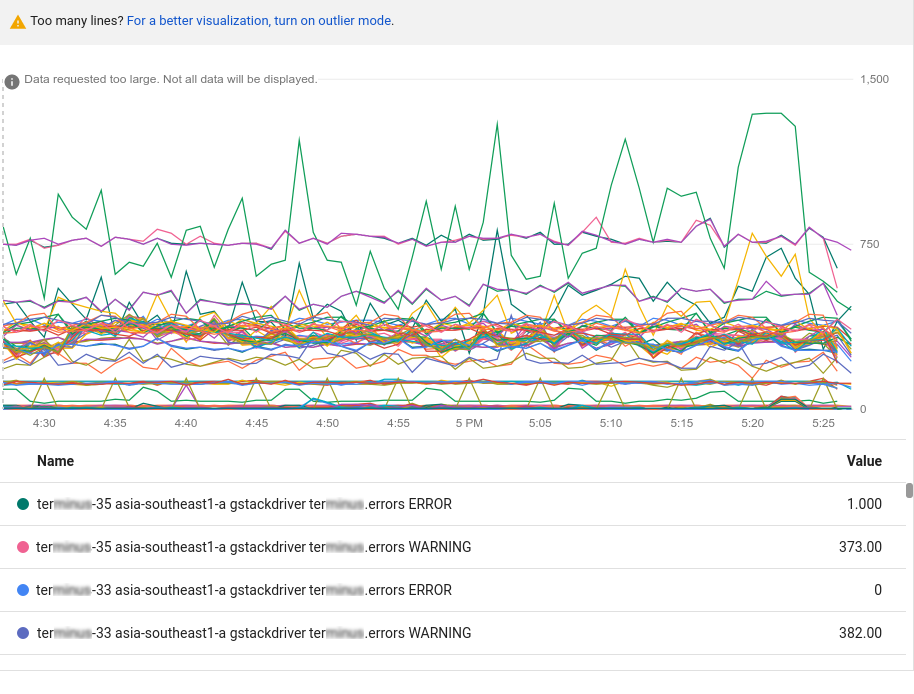
The previous chart contains more data than can be displayed; charts are
limited to 50 displayable lines.
The chart provides a notice that there is too much data to display. To
reduce the amount of data, in the query toolbar, use the
**Sort \& limit** element. For more information, see
[Show outliers](https://docs.cloud.google.com/monitoring/charts/working-with-charts#using-outlier-mode).
You can also use the filtering and aggregation options to reduce the amount
of charted data. These techniques make the charts more useful for
diagnostics and analysis, and they increase the performance and
responsiveness of the user interface itself.
4. Optional: Add filters to restrict which time series are shown. The next
section describes the filtering options.
5. Optional: Configure how the time series are grouped and aligned. For more
information, see [Choose how to display charted data](https://docs.cloud.google.com/monitoring/charts/metrics-selector#select_display).
#### Filter charted data
Filters ensure that only time series that meet some set of criteria are charted.
When you apply filters, you might reduce the number of lines on the chart,
which can improve the performance of the chart. Another way that you can improve
the responsiveness of a chart is to configure aggregation options, and to
sort and limit the number of time series that are displayed.
For more information, see [Show outliers](https://docs.cloud.google.com/monitoring/charts/working-with-charts#using-outlier-mode).
A filter is composed of a label, a comparator, and a value. For example,
to match all time series whose `zone` label starts with `"us-central1"`, you
could use the filter `zone=~"us-central1.*"`, which uses a regular expression
to perform the comparison. There are four comparator operators:
- equals, `=`
- not equals, `!=`
- regular expression match, `=~`
- regular expression does not match, `!=~`
When you filter by the project ID or the resource container,
you must use the equals operator, `(=)`. When you filter by
other labels, you can use any supported comparator.
Typically, you can filter metric and resource labels, and by
[resource group](https://docs.cloud.google.com/monitoring/groups).
When you supply multiple filtering criteria, the corresponding chart shows
only the time series that meet *all* criteria, a logical `AND`.
To add a filter when using the menu-driven interface of the Google Cloud console,
do the following:
1. In the **Filter** element, click **Add filter**, and make a selection
from the menu.
The menu lists user metadata labels, such as `user_labels`, only for
resources that exist in your project. To filter by labels for deleted
resources, write a PromQL query or a Monitoring-filter
query.
2. To change the comparison, select a value from the **Comparator** menu.
3. In the **Value** field, enter or select a value:
- For a direct comparison, `=` or `!=`, select the value from the
menu or enter a value and click **Ok** . You can enter values
such as `us-central1-a`, or you can create a filter
string that begins with `starts_with` or `ends_with`.
For example, to display data for any `us-central1` zone you could enter
the filter string `starts_with("us-central1")`.
See [Monitoring filters](https://docs.cloud.google.com/monitoring/api/v3/filters)
for more information on filter strings.
Because the menu entries are derived from the received time series, when
a monitored resource isn't generating data for the selected metric,
you must enter a value for the label.
- For a regular expression comparison, `=~` or `!=~`, enter a
[RE2](https://github.com/google/re2/wiki/Syntax)
regular expression into the **Value** field and click **Ok** .
For example, the regular expression
`us-central1-.*` matches all `us-central1` zones.
To match any US zone that ends with "a", you could use the
regular expression `^us.*.a$`.
You can't use regular expressions to filter the `project_id`
resource label.
For example, to view only the time series from one of the
`us-central1` zones, apply a `zone=~"us-central1.*"` filter.
When you add multiple filters, the following points apply:
- You can use the same label multiple times, which lets you
specify a filter for a range of values.
- All filter criteria must be met; they constitute a logical `AND`.
To edit the value or comparator for a filter,
on the filter element, click **Menu** , make your
changes, and then click **Ok**.
To delete a filter, click **Cancel**.
### Write PromQL queries
To enter a PromQL query, do the following:
1. In the Google Cloud console, go to the
**Metrics explorer** page:
[Go to **Metrics explorer**](https://console.cloud.google.com/monitoring/metrics-explorer)
If you use the search bar to find this page, then select the result whose subheading is
**Monitoring**.
2. In the toolbar of the Google Cloud console, select your Google Cloud project. For [App Hub](https://docs.cloud.google.com/app-hub/docs/overview) configurations, select the App Hub host project or management project.
3. In the toolbar of the query-builder pane, select the button whose name is **PromQL**.
4. Optional: Disable the **Auto-run** toggle.
5. Enter your query into the query editor. For example, to chart the average
CPU utilization of the VM instances in your Google Cloud project, use the
following query:
```
avg(compute_googleapis_com:instance_cpu_utilization)
```
For more information about using PromQL, see
[PromQL in Cloud Monitoring](https://docs.cloud.google.com/monitoring/promql).
6. Click **Run query**.
When the **Auto-run** toggle is enabled,
the **Run query** button isn't shown.
### Write Monitoring-filter queries
When you want to do any of the following, you must use *direct filter mode* ,
which lets you enter a
[Monitoring filter](https://docs.cloud.google.com/monitoring/api/v3/filters):
- Display a service-level objective (SLO).
- Display the count of processes running on virtual machines (VMs).
- Display a custom metric for which you don't yet have data.
- Filter a time series based on a label for which you don't yet have data.
A *Monitoring filter* , or equivalently a
*metric filter* , is an expression that Monitoring
uses to identify the time series to chart.
For example, the following expression results
in a chart displaying a count of processes whose name includes `nginx`:
select_process_count("monitoring.regex.full_match(\".*nginx.*\")")
resource.type="gce_instance"
You can also use Monitoring filters to identify time series
by their resource and metric type. The following expression results in a
chart displaying the count of log entries for all Google Cloud virtual
machine instances in the `us-east1-b` zone:
metric.type="logging.googleapis.com/log_entry_count"
resource.type="gce_instance"
resource.label."zone"="us-east1-b"
To enter a Monitoring filter, do the following:
1. In the Google Cloud console, go to the
**Metrics explorer** page:
[Go to **Metrics explorer**](https://console.cloud.google.com/monitoring/metrics-explorer)
If you use the search bar to find this page, then select the result whose subheading is
**Monitoring**.
2. In the toolbar of the Google Cloud console, select your Google Cloud project. For [App Hub](https://docs.cloud.google.com/app-hub/docs/overview) configurations, select the App Hub host project or management project.
3. Click **Help** on the **Metric** element, and then
select **Direct Filter Mode**.
The **Metric** and **Filter** elements are deleted, and a **Filters**
element lets you enter text, is created.
If you selected a resource type, metric,
or filters before switching to **Direct Filter Mode** mode, then
those settings are shown in the **Filters** element.
4. In the text area of the **Filters** element, enter
a Monitoring filter expression.
For syntax information, see the following documents:
- [Monitoring filters](https://docs.cloud.google.com/monitoring/api/v3/filters)
- [Process-health filters](https://docs.cloud.google.com/monitoring/api/v3/process-health-filters)
- [Retrieving SLO data](https://docs.cloud.google.com/stackdriver/docs/solutions/slo-monitoring/api/timeseries-selectors)
When you use direct filter mode and no data is available that satisfies the
filter, an error is shown. Common error messages include
`Chart definition invalid` and
`No data is available for the selected timeframe.`
5. Optional: Configure how the time series are grouped and aligned. For more
information, see [Choose how to display charted data](https://docs.cloud.google.com/monitoring/charts/metrics-selector#select_display).
To return to the menu-driven interface,
click **Exit direct filter mode**.
> [!NOTE]
> **Note:** If you enter an Monitoring filter and then switch to a different interface, the Monitoring filter is discarded.
## Choose how to display charted data
This section covers how to display the selected data by setting the
aggregation fields. Aggregation consists of alignment of data points within
a time series, and combining different time series together.
For a detailed explanation of aggregation, see
[Filtering and aggregation: manipulating time series](https://docs.cloud.google.com/monitoring/api/v3/aggregation).
- For information on view options, see [Set chart display options](https://docs.cloud.google.com/monitoring/charts/chart-view-options).
- For more information about interacting with the chart itself, see [Explore charted data](https://docs.cloud.google.com/monitoring/charts/working-with-charts).
The content of this section doesn't apply when you've selected the data
to chart by using PromQL.
### Combine time series
You can reduce the amount of data returned for a metric by combining
different time series. To combine multiple time series, you typically
specify one or more labels and a function. Time series that have the
same value for all specified labels are grouped, and then the function
that you specified combines those time series into a new time series.
The settings in the **Aggregation** element can change the number of
time series that your chart displays. The default settings for the this element
are determined by the metric type you selected.
To modify the display, do any of the following:
- To display every time series, in the **Aggregation** element,
ensure the first menu is set to **Unaggregated** and the second menu is
set to **None**.
- To combine time series, in the **Aggregation** element,
do the following:
1. Expand the first menu and select a function.
The chart is refreshed and displays a single time series. For example,
if you select **Mean**, then the displayed time series is the average
of all time series.
The function menu supports common algebraic functions, like mean, minimum,
maximum, and sum. The **Count time series** option counts the number of
time series that match the metric and filter settings. The
percentile options, like **99th percentile**, are statistical values
derived from the time series that match the metric and filter settings.
2. To combine time series that have the same label values,
expand the second menu, and then select one or more labels.
The chart is refreshed and shows one time series for each unique
combination of label values. For example, to display on time series
per zone, set the second menu to **zone**.
- To configure the spacing between data points, click
**Add query element** , select **Min Interval**,
and then enter a value.
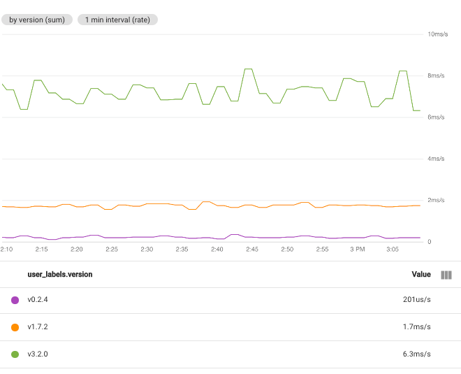
For example, if you set the function to **Sum** and select the label
**user_labels.version** , then there is one time series for
each value of the label **user_labels.version**.
The data points in each time series are computed from the sum of all the values
for individual time series for a specific version:
When you select multiple labels, time series that have the same
values for the selected labels are combined.
The resulting chart displays one time series for each combination of label
values. The order in which you specify the labels doesn't matter.
The following screenshot shows a chart where time series are combined by the
**user_labels.version** and **system_labels.machine_image** labels:
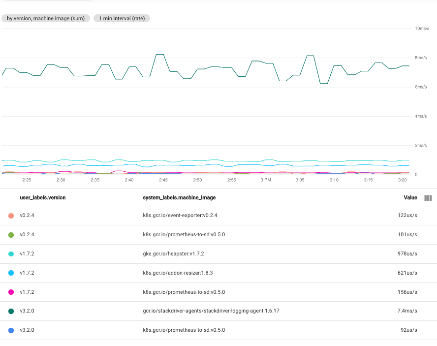
As shown, the chart displays one time series for each pair of label values.
The fact that you get a time series for each combination of labels means that
this technique can create more data than you can usefully put on a
single chart.
#### Show all time series
To show all time series, on the **Aggregation** element,
set the first menu to **Unaggregated** and the second menu to **None**.
### Align time series
Alignment is the process of converting the time series data received by
Monitoring into a new time series which has data points at
fixed intervals. The process of alignment consists of collecting all data
points received in a fixed length of time, applying a function to combine
those data points, and assigning a timestamp to the result. That
function might compute the average of all samples or
it might extract the maximum of all samples.
#### Set alignment interval
To specify the fixed length of time for points to be combined,
click **Add query element** in the query pane,
select **Min Interval**, and then complete the dialog.
For example, consider a metric with a sampling period of one minute. If a chart
is configured to display 1 hour of data, then the chart can display all 60 data
points. If the **Min Interval** field is set to `10 minutes`, then the
chart displays 6 data points. However, if you now configure the chart to display
one week of data, then there are too many points to display in the chart so the
the interval over which points are combined is automatically modified.
In this example, the modified interval is one hour.
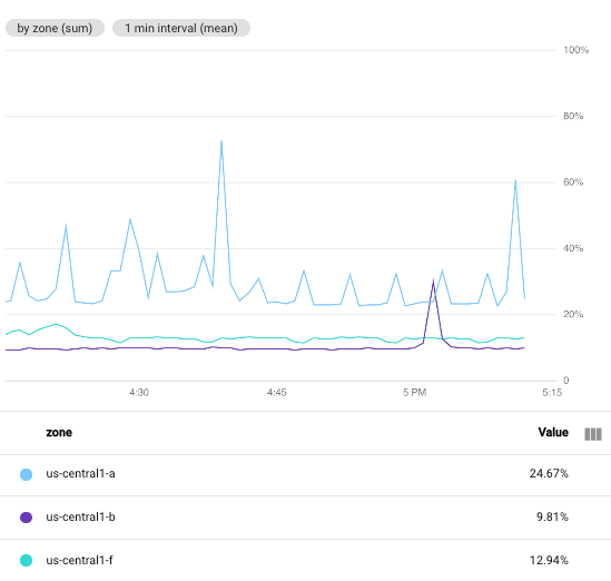
The following screenshot illustrates the CPU utilization of the
Compute Engine VM instances in a particular Google Cloud project.
In this image, the **Min Interval** field is set to `1 minute`:
For comparison, the following screenshot illustrates the effect of changing
the interval from `1 minute` to `5 minutes`:
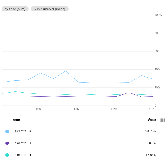
By increasing the period, the resulting chart has fewer points, decreasing from
60 points per time series to 10 points per time series. By increasing the
**Min Interval** field, more points are combined, which has a smoothing
effect on the plotted data.
#### Set alignment function
When you select the function for aggregation, Cloud Monitoring selects
the alignment function for you. Cloud Monitoring determines the optimal
alignment function based on the metric type you selected and your choice
for the aggregation function. However, you can specify an alignment function
and override the choice made by Cloud Monitoring.
To specify the alignment function,
do the following:
1. In the **Aggregation** element, expand the first menu and select **Configure aligner** . The **Alignment function** and **Grouping** elements are added.
2. Expand the **Alignment function** element and make a selection.
While most of the supported alignment functions perform common
mathematical functions, some perform more complicated actions:
- **next older** : To retain only the most recent sample within an alignment
period, select **next older**. This function is commonly used with
uptime checks and is a good choice when you only care about the most recent
value.
This function is valid only for gauge metrics.
- **percentile**: To display a distribution metric on a plot type of line
chart, stacked area chart, or stacked bar chart, you must select which
percentile in the distribution to display. One way to specify this percentile
is to select a percentile function. You can select the 5th, 50th, 95th, and
the 99th percentiles. The aligned data point is determined by computing the
specified percentile by using all data points in the alignment period.
This function is valid only for gauge and delta metrics when they
have a distribution data type.
- **delta** : To convert a cumulative metric or a delta metric into a delta
metric with one sample per alignment period, use this function.
Data interpolation might occur when you use this function.
For an example, see
[Kinds, types, and conversions](https://docs.cloud.google.com/monitoring/api/v3/aggregation#ts-conversion).
This function is valid only for cumulative and delta metrics.
- **rate** : To convert a cumulative or delta metric into a gauge metric, use
this function. If you choose this function, you can think of the time series
being transformed as it was with a delta function and then divided by
the alignment period. For example, if the unit of the original time series
is MiB and the unit of the alignment period is second, then the
chart has a unit of MiB per second. For more information, see
[Kinds, types, and conversions](https://docs.cloud.google.com/monitoring/api/v3/aggregation#ts-conversion).
This function is valid only for cumulative and delta metrics.
For more information on the available alignment functions,
see [`Aligner`](https://docs.cloud.google.com/monitoring/api/ref_v3/rest/v3/projects.alertPolicies#Aligner)
in the API reference.
### Secondary grouping and alignment
When you have multiple time series that already represent aggregations,
you can reduce all the time series on the chart to a single
time series by choosing a **Secondary Aggregator**. For example, if you
group data by zone, your chart shows one time series for each zone. To
create a chart with a single time series, use the secondary aggregation
fields.
For some metric types, you have the option to transform the data. If this
option is available and if you set the **Transform** field to a value other
than **None**, all other fields are the secondary aggregation settings.
When the secondary aggregation fields are configurable, to access those fields,
to the following:
1. Click **Add query element** , and then select **Secondary aggregation**.
2. Configure the **Secondary aggregation** element.
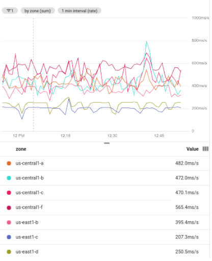
The following screenshot shows several time series that result from
grouping a filtered set of data. The use of grouping requires aggregation;
each group of lines is aggregated into one. The following screenshot shows
time series grouped by zone:
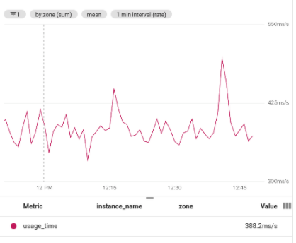
The following screenshot shows the result of using secondary aggregation to
find the mean value across the grouped time series:
## Configure the name of a legend column
The **Legend Alias** field lets you customize a description for the
time series on your chart. These descriptions appear on the tooltip for
the chart and on the chart legend in the **Name** column.
By default, the descriptions in the legend are created for you from the values
of different labels in your time series. Because the system selects the
labels, the results might not be helpful to you. To build a template for
descriptions, use this field.
You can enter plain text and templates in the **Legend Alias** field. When
you add a template, you add an expression that is evaluated when the legend
is displayed.
To add a legend template to a chart, do the following:
1. In the **Display** pane, expand **Legend Alias**.
2. Click **Display template variable suggestions** and select an entry from the menu. For example, if you select `zone`, then the template `${resource.labels.zone}` is added.
For example, the following screenshot shows a legend template that contains
plain text and the expression `${resource.labels.zone}`:

In the chart legend, the values generated from the template appear in a column
with the header **Name** and in the tooltip:
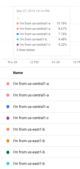
You can configure the legend template to include multiple text strings and
templates; however, the display space available on the tooltip is limited.
## What's next
- [Explore charted data](https://docs.cloud.google.com/monitoring/charts/working-with-charts)
- [User-defined metrics overview](https://docs.cloud.google.com/monitoring/custom-metrics)
- [Configure the legend template](https://docs.cloud.google.com/monitoring/charts/working-with-legends#descr_template)
- [Set chart display options](https://docs.cloud.google.com/monitoring/charts/chart-view-options)