Metric widgets on a custom dashboard in Cloud Monitoring let you track
time-series trends and monitor the latest values of your
[metric data](https://docs.cloud.google.com/monitoring/api/v3/metrics), including [user-defined](https://docs.cloud.google.com/monitoring/custom-metrics) and
[log-based](https://docs.cloud.google.com/logging/docs/view/logs_based_metrics) metrics. You can visualize this data over time
using line, stacked area, stacked bar, or heatmap charts, or display the most
recent values using tables, gauges, scorecards, histograms, pie charts, and
treemaps.
For information about how to display other types of data on your custom
dashboards, such as log data or text, see the [What's next](https://docs.cloud.google.com/monitoring/charts#whats-next)
section of this document. To configure custom dashboards
programmatically, see [Manage dashboards by API](https://docs.cloud.google.com/monitoring/dashboards/api-dashboard).
## Visualizations for metric data
To display data over time, use **Charts**. There are four styles available:
- Line
- Stacked area
- Stacked bar
- Heatmap
Line charts are the default visualization and are suitable for most metric data.
Stacked bar charts are best when you are charting metric data that has
infrequent samples, such as quota metrics. For metric data whose value type is a
distribution, use the heatmap.
To display only the most recent values, use one of the following styles:
- [Tables](https://docs.cloud.google.com/monitoring/charts#add_table) display labels, let you limit the number of rows, and let you color-code cells based on the value.
- [Gauges](https://docs.cloud.google.com/monitoring/charts#add_gauge_scorecard) and [Scorecards](https://docs.cloud.google.com/monitoring/charts#add_gauge_scorecard) display a green, amber, or red indication based on how the value compares to a set of thresholds.
- [Histograms](https://docs.cloud.google.com/monitoring/charts#add_histogram) display the relative frequency of the most recent values of multiple time series.
- [Pie charts](https://docs.cloud.google.com/monitoring/charts#add_pie) display the most recent value of each time series as a fraction of the sum of all values.
- [Treemaps](https://docs.cloud.google.com/monitoring/charts#add_treemap) display the most recent values of grouped data as a series of nested rectangles, where the color for a rectangle is proportional to its value.
After a widget is configured, you can
[change its visualization](https://docs.cloud.google.com/monitoring/charts#visualization).
## Before you begin
Complete the following in the Google Cloud project where you want to create and
manage dashboards:
-
To get the permissions that
you need to create and modify custom dashboards by using the Google Cloud console,
ask your administrator to grant you the
[Monitoring Editor](https://docs.cloud.google.com/iam/docs/roles-permissions/monitoring#monitoring.editor) (`roles/monitoring.editor`) IAM role on your project.
For more information about granting roles, see [Manage access to projects, folders, and organizations](https://docs.cloud.google.com/iam/docs/granting-changing-revoking-access).
You might also be able to get
the required permissions through [custom
roles](https://docs.cloud.google.com/iam/docs/creating-custom-roles) or other [predefined
roles](https://docs.cloud.google.com/iam/docs/roles-overview#predefined).
For more information about roles, see
[Control access with Identity and Access Management](https://docs.cloud.google.com/monitoring/access-control).
- You can put up to 100 widgets on a dashboard.
## Display metric data on a dashboard
To display metric data on your dashboard, complete the following steps:
1. [Open a dashboard and add a widget](https://docs.cloud.google.com/monitoring/charts#open)
2. [Select a metric type to display](https://docs.cloud.google.com/monitoring/charts#select-data)
3. [Save your changes](https://docs.cloud.google.com/monitoring/charts#save)
You might want to change the appearance of the chart, display a ratio of
metrics, or make other changes. To learn about the available options, see the
[Advanced configuration options](https://docs.cloud.google.com/monitoring/charts#advanced) section of this document.
### Open a dashboard and add a widget
To display metric data on a custom dashboard, do the following:
1. In the Google Cloud console, go to the **Dashboards** page:
[Go to **Dashboards**](https://console.cloud.google.com/monitoring/dashboards)
If you use the search bar to find this page, then select the result whose subheading is
**Monitoring**.
2. In the toolbar of the Google Cloud console, select your Google Cloud project. For [App Hub](https://docs.cloud.google.com/app-hub/docs/overview) configurations, select the App Hub host project or management project.
3. Do one of the following:
- To create a new dashboard, select **Create dashboard**.
- To update an existing dashboard, find the dashboard in the list of all dashboards and select its name.
4. In the toolbar, click **Add widget**.
5. In the **Add widget** dialog, select a widget.
- To add a line chart, select **Metric**.
- To add a different visualization, select the visualization from the widget library.
You can [change the visualization style](https://docs.cloud.google.com/monitoring/charts#visualization) by
using widget options.
### Select a metric type to display
In this step, you configure a query. The query defines what data the widget
displays.
### Menu-driven interface
1. Select the time series data that you want to view:
1. In the **Metric** element, expand the **Select a metric** menu.
The **Select a metric** menu contains features that help you find
the metric types available:
- To find a specific metric type, use the **Filter bar** . For example, if you by enter `util`, then you restrict the menu to show entries that include `util`. Entries are shown when they pass a case-insensitive "contains" test.
- To show all metric types, even those without data, click **Active**. By default, the menus only show metric types with data.
For example, you might make the following choices:
1. In the **Active resources** menu, select **VM instance**.
2. In the **Active metric categories** menu, select **uptime_check**.
3. In the **Active metrics** menu, select **Request latency**.
4. Click **Apply**.
2. Optional: To specify a subset of data to display, in the **Filter** element, select **Add filter** , and then complete the dialog. For example, you can view data for one zone by applying a filter. You can add multiple filters. For more information, see [Filter charted data](https://docs.cloud.google.com/monitoring/charts/metrics-selector#filter-option).
For more information, see [Select the data to chart](https://docs.cloud.google.com/monitoring/charts/metrics-selector).
2. Combine and align time series:
- To display every time series, in the **Aggregation** element, set the first menu to **Unaggregated** and the second menu to **None**.
- To combine time series, in the **Aggregation** element, do the following:
1. Expand the first menu and select a function.
The chart is refreshed and displays a single time series. For
example, if you select **Mean**, then the displayed time series is
the average of all time series.
2. To combine time series that have the same label values,
expand the second menu, and then select one or more labels.
The chart is refreshed and shows one time series for each unique
combination of label values. For example, to display on time series
per zone, set the second menu to **zone**.
When the second menu is set to **None**, the chart displays one
time series.
- Optional: To configure the spacing between data points, click **Add query element** , select **Min Interval**, and then enter a value.
For more information about grouping and alignment, see
[Choose how to display charted data](https://docs.cloud.google.com/monitoring/charts/metrics-selector#select_display).
3. Optional: To display only the time series with the highest or lowest values, use the **Sort \& Limit** element.
### PromQL
1. In the toolbar of the query-builder pane, select the button whose name is **PromQL**.
2. Enter your query into the query editor. For example, to chart the average
CPU utilization of the VM instances in your Google Cloud project, use the
following query:
```
avg(compute_googleapis_com:instance_cpu_utilization)
```
For more information about using PromQL, see
[PromQL in Cloud Monitoring](https://docs.cloud.google.com/monitoring/promql).
### Monitoring filter
1. In the **Metric** element, click **Help** , and then
select **Direct Filter Mode**.
The **Metric** and **Filter** elements are deleted, and a **Filters**
element that lets you enter text, is created.
If you selected a resource type, metric,
or filters before switching to **Direct Filter Mode** mode, then
those settings are shown in the field of the **Filters** element.
2. Enter a Monitoring filter in the field of the **Filters** element.
3. Combine and align time series:
- To display every time series, in the **Aggregation** element, set the first menu to **Unaggregated** and the second menu to **None**.
- To combine time series, in the **Aggregation** element, do the following:
1. Expand the first menu and select a function.
The chart is refreshed and displays a single time series. For
example, if you select **Mean**, then the displayed time series is
the average of all time series.
2. To combine time series that have the same label values,
expand the second menu, and then select one or more labels.
The chart is refreshed and shows one time series for each unique
combination of label values. For example, to display on time series
per zone, set the second menu to **zone**.
When the second menu is set to **None**, the chart displays one
time series.
- Optional: To configure the spacing between data points, click **Add query element** , select **Min Interval**, and then enter a value.
For more information about grouping and alignment, see
[Choose how to display charted data](https://docs.cloud.google.com/monitoring/charts/metrics-selector#select_display).
### Save your changes
After you select a metric type to display, you can save your changes,
change the default settings, or configure widget-specific fields.
The following sections of this document might be helpful when you
configure widget-specific fields:
- [Configure a table](https://docs.cloud.google.com/monitoring/charts#add_table)
- [Configure gauges and scorecards](https://docs.cloud.google.com/monitoring/charts#add_gauge_scorecard)
- [Configure histograms, pie charts, and treemaps](https://docs.cloud.google.com/monitoring/charts#configure-other)
When you are satisfied with your chart, save the changes and then
update the dashboard.
1. To apply your changes to the dashboard, in the toolbar, click **Apply** . To discard your changes, click **Cancel**.
2. To save your modified dashboard, in the toolbar, click **Save**.
After you save your widget, you can edit that widget and modify any of its
settings. For example, you can change the visualization style.
## Advanced configuration options
This section describes the options available to you to customize your widget:
- [Change the visualization](https://docs.cloud.google.com/monitoring/charts#visualization)
- [Set appearance](https://docs.cloud.google.com/monitoring/charts#appearance)
- [Set visibility](https://docs.cloud.google.com/monitoring/charts#visibility)
- [Set the time range](https://docs.cloud.google.com/monitoring/charts#time-range-override)
- [Display multiple metric types](https://docs.cloud.google.com/monitoring/charts#multiple-metrics)
- [Display a ratio of metric types](https://docs.cloud.google.com/monitoring/charts#ratio)
### Change the visualization
To display the most recent values of your metric data, instead of displaying
that data over time, use one of the following visualizations:
- [Table](https://docs.cloud.google.com/monitoring/charts#add_table)
- [Gauge](https://docs.cloud.google.com/monitoring/charts#add_gauge_scorecard)
- [Scorecard](https://docs.cloud.google.com/monitoring/charts#add_gauge_scorecard)
- [Histogram](https://docs.cloud.google.com/monitoring/charts#add_histogram)
- [Pie](https://docs.cloud.google.com/monitoring/charts#add_pie)
- [Treemap](https://docs.cloud.google.com/monitoring/charts#add_treemap)
To modify your widget's visualization, in the **Display** pane,
select **Widget type** and make a selection from the menu.
The **Widget type** menu lists all widget types that can display the same type
of data; however, some widgets might not be enabled.
For example, suppose a line chart displays several time series. The
**Widget type** menu shows that most visualization types are listed as
**Compatible**. For example, you can always switch from a line chart to a table.
However, the following widget types aren't available:
- The **Heatmap** widget is disabled because these widgets can only display distribution-valued data.
- The logs panel isn't listed because the logs panel can't display metric data.
### Set appearance
Optional: To change how a chart or table displays the selected data, use the
options in the **Display** pane:
- Chart options:
- [**Analysis mode** menu](https://docs.cloud.google.com/monitoring/charts/chart-view-options#chart-modes): Select between line charts, x-ray, and statics.
- [**Compare to Past** menu](https://docs.cloud.google.com/monitoring/charts/working-with-charts#comparetopast-option): Overlay current data with past data.
- [**Threshold Line** menu](https://docs.cloud.google.com/monitoring/charts/working-with-legends#descr_template): Add a reference threshold.
- [**Legend Alias** menu](https://docs.cloud.google.com/monitoring/charts/working-with-legends#descr_template): Configure the name of a legend column.
- [**Y-axis assignment** , **Y-axis labels** , and **Y-axis scale** menus](https://docs.cloud.google.com/monitoring/charts/chart-view-options#logscale-option): Configure configure Y-axis assignment, labels, or scale.
- Table options:
- [**Value option** menu](https://docs.cloud.google.com/monitoring/charts#display-latest-or-aggregated): Select between the latest value and an aggregated value.
- [**Visible columns** menu](https://docs.cloud.google.com/monitoring/charts#configure-visible-columns): Select which columns are shown.
- [**Column formatting** menu](https://docs.cloud.google.com/monitoring/charts#configure-columns): Configure column names, alignment of data in a column, units, and whether cells are color-coded.
- [**Metric view** menu](https://docs.cloud.google.com/monitoring/charts#reference-value): Select whether the value is show by itself or shown relative to a range of values.
- [**Legend Alias** menu](https://docs.cloud.google.com/monitoring/charts/working-with-legends#descr_template): Configure the name of a legend column.
### Set visibility
By default, your dashboard displays your widget. If you define
[variables](https://docs.cloud.google.com/monitoring/dashboards/filter-permanent), then you can make your widget visible only
when the variable has specific values. For more information, see
[Set the visibility of a widget](https://docs.cloud.google.com/monitoring/dashboards/filter-permanent#set-visibility).
### Set the time range
The time-range setting shown by a dashboard's toolbar applies to every widget
on the dashboard, with the following exceptions:
- Widgets whose query specifies the time range.
- Widgets that configure a time-range override. This override is available for most charts. However, it isn't available for charts that display data monitored by an alerting policy or for non-chart widget types such as tables.
Configure a chart's time-range override when you want that chart to show data
over a longer or shorter time range than is appropriate for other dashboard
widgets. For example, consider these use cases:
- A dashboard displays a quota metric, which has 1 sample per day, and metric
data that is sampled every 60 seconds. The quota-metric chart needs a
time range of at least one day, possibly as long as one week. However, this
time range is too long to view spikes or dips in the metrics that
are sampled every 60 seconds.
- For a metric, you want to view both trends and the current measurements.
Therefore, you add two charts to the dashboard. For one chart, you set
its time-range override to eight days, a bit longer than a week. The other
chart displays one hour of data, which is the dashboard's time-range
setting.
To configure the chart to override the dashboard setting, in the **Display**
pane, expand the **Time Range Override** field, and then complete the dialog.
You can enter either a relative time range or an absolute time range.
### Display multiple metric types
You can configure charts and tables to display multiple metric types.
For tables, Cloud Monitoring tries to display the values for both
metric types on the same row, when possible. For more information, see
[How tables merge data from multiple metric types](https://docs.cloud.google.com/monitoring/charts#table-multiple-metric).
### Menu-driven interface
1. Select **Add query** . A new query is added. For example, a query with the label **B** might be added.
2. For the new query, in the **Metric** element, select a resource type and metric type. You can also add filters, combine time series, and sort and limit the number of displayed time series.
The following screenshot illustrates the Metrics Explorer display when
there are two metric types charted:

### PromQL
Not supported.
### Monitoring filter
Not supported.
### Display a ratio of metric types
You might want to chart a ratio of metrics when Google Cloud doesn't
provide the metric data in the form you prefer.
### Menu-driven interface
1. Configure the chart to display two metric types that have the same metric kind. For example, both are `GAUGE` metrics.
2. Ensure that the value of the **Min Interval** field is the same for both metric types. To access this field, click **Add query element** and select **Min Interval**.
3. Update the aggregation fields.
We recommend that the labels for the denominator metric type match the values
set for the numerator metric type. For example, you might select the
`zone` label for the numerator and denominator.
You aren't required to use the same set of labels for both metric types;
however, you can only select labels that are common to both metric types.
4. In the toolbar of the query pane, select **Create ratio**, and then
complete the dialog.
After you create the ratio, three queries are shown:
- **A/B Ratio** identifies the ratio query.
- **A** identifies the query for the numerator.
- **B** identifies the query for the denominator.
The following example illustrates a ratio that compares the sum of
the bytes written to disk per zone, to the total number of bytes
written to disk:

5. Optional: To switch the numerator and denominator metrics, in the
**Ratio** element, expand the menu, and then make a selection.
### PromQL
1. In the toolbar of the query-builder pane, select the button whose name is **PromQL**.
2. Enter your query into the query editor. For example, to chart the ratio of
average latency of your `my_summary_latency_seconds` metric, use the
following query:
```
sum without (instance)(rate(my_summary_latency_seconds_sum[5m])) /
sum without (instance)(rate(my_summary_latency_seconds_count[5m]))
```
For more information about using PromQL,
see [PromQL in Cloud Monitoring](https://docs.cloud.google.com/monitoring/promql).
### Monitoring filter
Not supported.
## Configure a table
To view the most recent data in tabular form, add a table.
Tables can display numeric data. For example, they can display one or more
[metric types](https://docs.cloud.google.com/monitoring/api/v3/metrics),
or percentiles for distribution-valued metrics.
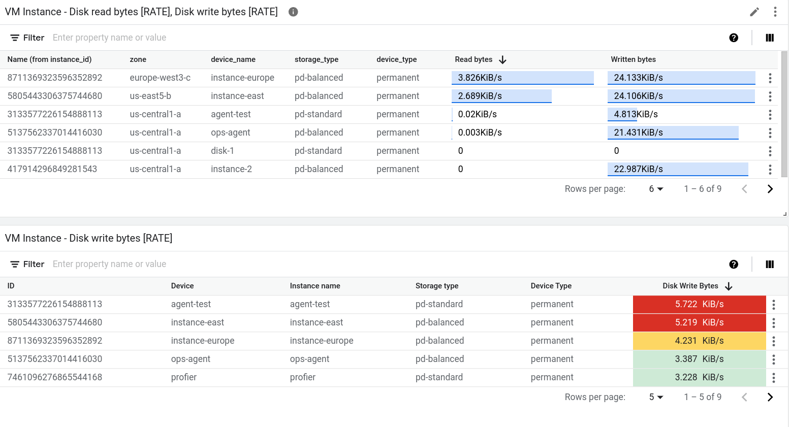
The following screenshot illustrates two tables. The first table displays two
metric types, the number of bytes read from instances and the number of bytes
written to instances. An aggregated value is shown along with a reference bar.
The second table shows the latest value of one metric type,
and the value column has been configured to color-code the cell based on
how the value compares to a threshold:
There are two widgets that display data in tabular form: the **Top List** widget
and the **Table** widget. The primary difference between these two widgets is
that the **Top List** widget sorts the order of the rows, and it displays the
value along with a visual indicator of the value compared to the range of
possible values. Because the **Top List** widget provides a visual
representation of the value, you can't color-code the cell based on
how the value compares to a threshold.
To add a table to a dashboard, do the following:
1. [Open a dashboard and add a widget](https://docs.cloud.google.com/monitoring/charts#open).
2. In the widget menu, select **Table** or **Top List**.
3. [Select a metric type to display](https://docs.cloud.google.com/monitoring/charts#select-data).
Each row in the table corresponds to one time series. One table column
displays a numeric value that is either the latest value or an aggregate
value. The other columns display the labels in the time series.
4. Optional: Select another metric type.
When a table displays multiple metric types, the data for all metric types
is shown on the same row, when possible. For more information, see
[Understand tables that display multiple metric types](https://docs.cloud.google.com/monitoring/charts#table-multiple-metric).
5. Configure the table:
- [Display latest value or aggregated value](https://docs.cloud.google.com/monitoring/charts#display-latest-or-aggregated).
- [Select the columns to display](https://docs.cloud.google.com/monitoring/charts#configure-visible-columns).
- [Configure columns](https://docs.cloud.google.com/monitoring/charts#configure-columns).
- [Display referential value](https://docs.cloud.google.com/monitoring/charts#reference-value).
- [Sort and filter tables](https://docs.cloud.google.com/monitoring/charts#sort-filter).
You can also use the Cloud Monitoring API to add a table widget to a
dashboard. For more information, see
[Dashboard with a `TimeSeriesTable` widget](https://docs.cloud.google.com/monitoring/dashboards/api-examples#dashboard_with_a_table_widget).
### Display latest value or aggregated value
By default, tables display the most recent value. However, a table can
show a value that is computed over the time range selected for
your dashboard.
To select between the latest value and the aggregated value, use the
**Value option** field.
If you display the aggregated value, then for each time series, the data
within the time range selected by your dashboard is combined by the
alignment function. The alignment function is one of the aggregation options
and isn't shown by default. To view the alignment function, expand the
**Aggregation** element, and in the first element, select **Configure aligner** .
After you make this selection, the **Aggregation** element is replaced
by a **Grouping** element and a menu named **Alignment function**.
### Select the columns to display
By default, one column in the table displays a numeric value. All other
columns correspond to a label in the time series. For label-based columns,
the column name is derived from the label.
To configure the columns shown by the table, expand the **Visible Columns**
menu and make your selections.
> [!NOTE]
> **Note:** Ensure that you select the column that displays the numeric value.
### Configure column format
- To configure an individual column, in the **Columns** element,
expand the **Override column** menu, select the column to be modified, and
then do any of the following:
- To set the name of the column, use the **Display name** field.
- To set the alignment of the data in the column, use the **Left align** , **Center align** , and **Right align** buttons.
- To color-code the cell based on how the numeric value compares to a threshold, set the warning and danger thresholds.
- If you write PromQL queries, then use the **Unit** menu to set the units shown with the data. The units are automatically configured when you configure your query by using menu selections.
### Display referential value
> [!NOTE]
> **Note:** You can't use this option when you've configured a column to color-code a cell based on the numeric value in the cell.
Tables can display only a value, or they can display a value relative to
the range of values. When the range option is selected, the value is shown
along with a blue-colored bar; the length of the bar is proportional to the
value shown.
To configure whether a referential value is shown, use the **Metric view**
element.
### Sort and filter
You can change the order of the rows in the table display, and you can
filter the table contents so that only specific rows are shown.
These settings aren't persistent. When you leave the dashboard page or when
you reload the dashboard, the sorting and filtering options you applied are
discarded.
You have the following sorting and filtering options:
- To sort the table by a column, click the column header.
- To change the table columns, click **View columns** ,
make your modifications, and then click **OK**.
- To list only specific rows, add one or more filters. You can add multiple
filters. When you don't specify the OR operator between two filters, a
logical-AND joins those filters.
To add a filter, click `Enter property name or value`, select a
property from the menu, and then enter a value or select from the value
menu. For example, if you filter on the property `Name` and enter the value
`demo`, then the table lists only rows where the `Name` field
*includes* the value `demo`.
### Understand tables that display multiple metric types
If a table queries for multiple metric types, then the Google Cloud console
performs a merge operation by examining the labels attached to the aggregated
data for both metric types. When the labels that are common to both queries
let Monitoring determine a unique row identifier, then a
single row on the table displays the most recent value for each query.
Otherwise, there is one row for each time series.
For example, suppose a table queries two different metric types. Let's call
these queries `A` and `B`. The following describes how the query results
are merged:
- If the result of both queries has the same set of labels, then the merge is
always successful. Each row contains the latest value for each query.
If a query doesn't return a value for a particular combination of labels,
then the table cell is empty.
For example, suppose both queries contain a `zone` label. The table
contains one row for each zone reported by query `A` and query `B`.
However, if query `A` returns a time series whose zone is `us-central1-a`
but query `B` doesn't return a time series with this value, then the
latest value for query `B` is shown as an empty cell.
- If the labels for the results of one query are a subset of the labels for
the results of the other query, then the results are merged.
For example, suppose that results for both queries include labels for
`location` and `cluster_name`, but that the results for query `A` also
include a label for `memory_type`. In this situation, each row corresponds
to a time series with unique values for the three labels.
On any row, the value shown for query `B` is the value of the time series
that matches the two common labels, `location` and `cluster_name`, and
the third label is ignored.
- If the results of the two queries don't share any labels or if they
share some labels, but not enough to form a unique row identifier,
then the results can't be merged.
The table lists one row for each time series
returned by query `A` or by query `B`, and some table cells are empty.
For example, suppose the labels for query `A` are `location` and
`memory_type`, and that the labels for query `B` are `location` and
`cluster_name`. Even though the label `location` is common, that label isn't
sufficient to create a unique row identifier.
As described in the next section, you might be able to resolve a merge
failure.
#### How to resolve a merge failure
When you are charting multiple metrics, a merge failure might occur
because the metrics use different label names for the same field.
One way you can resolve this failure is to convert one query to PromQL
and then use the [`label_replace()`](https://prometheus.io/docs/prometheus/latest/querying/functions/#label_replace) function to
convert the label names used by one metric type to match those of the
other metric type.
For example, consider a table configured with two queries:
- `A`: Queries the `Prometheus/kube_pod_container_status_ready/gauge`
metric type. The aggregation options are set to sum time series after
grouping the data by the `cluster` label.
- `B`: Queries the `kubernetes.io/container/memory/request_bytes`
metric type. The aggregation options are set to sum time series after
grouping the data by the `cluster_name` label.
The table can't merge the results because the results for query `A` and
query `B` have different labels.
To resolve the failure, convert query `A` to PromQL and replace `cluster`
with `cluster_name`. The following example illustrates the modified query:
sum by (cluster_name)(
label_replace(
avg_over_time(kube_pod_container_status_ready[${__interval}]),
"cluster_name", "$1", "cluster", "(.*)"
)
)
With the changes, both queries produce the same set of labels.
Therefore, each row in the table lists a cluster name,
the value for query `A`, and the value for query `B`.
For information about using PromQL,
see [PromQL in Cloud Monitoring](https://docs.cloud.google.com/monitoring/promql).
## Configure gauges and scorecards
To view the most recent measurement as compared to a color-coded set of
thresholds, add a gauge or a scorecard. Gauges display only the most recent
measurement, while scorecards also show a history of recent measurements.
The background color of these widgets is also color-coded. When the most
recent value is within expected ranges, the widget color is white. When
the value is in a warning range, the widget becomes amber. Similarly, when the
value is in a danger range, the widget becomes red.
These widgets can display multiple gauges or scorecards. For example, the
following image shows a gauge widget that displays three gauges:
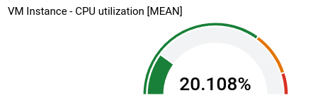
The number of gauges shown by the gauge widget depends on your aggregation
settings. In the example, the aggregation settings result in three time series,
so three gauges are shown. You define the thresholds at the widget level, so
they apply to each time series. In this example, one gauge is red, one is amber,
and the third is green.
The remainder of the information in this section is for the
Google Cloud console. For information about using the Cloud Monitoring API,
see [Dashboard with a basic `Scorecard`](https://docs.cloud.google.com/monitoring/dashboards/api-examples#basic-scorecard).
To add a gauge or scorecard to a dashboard, do the following:
1. [Open a dashboard and add a widget](https://docs.cloud.google.com/monitoring/charts#open).
2. In the widget menu, select **Gauge** or **Scorecard**.
3. [Select a metric type to display](https://docs.cloud.google.com/monitoring/charts#select-data).
> [!NOTE]
> **Note:** By default, when you add a **Gauge** or **Scorecard** widget to a dashboard, the queried time series are combined. If you want to display multiple gauges, as is shown in the previous example, then modify your aggregation settings. For example, you might group time series by zone.
4. In the **Display** pane, configure the widget:
1. For gauge widgets, click **Gauge range**,
and then set the minimum and maximum values. When a gauge displays a
percentage, set these values to 0 and 1, respectively.
2. Click **Gauge threshold**,
and then set the warning and danger thresholds. Threshold fields that
are empty aren't used.
For the gauge displayed previously, two thresholds are set. Values
higher than 0.9 are in the danger range. Values higher than 0.7 but
not in the danger range are in the warning range.
3. For scorecards, click **Spark chart view**,
then expand the menu of options, and then select the display style.
5. To apply your changes to the dashboard, in the toolbar,
click **Apply** . To discard your changes, click **Cancel**.
6. To save your modified dashboard, in the toolbar, click **Save**.
## Configure histograms, pie charts, and treemaps
This section provides information about how to configure widgets that show
the most recent metric values in a graphical form.
### Configure a histogram
A histogram provides information about the relative frequency of the
most recent value of multiple time series. That is, the x-axis
is indexed by *bins* , each of which corresponds to a range of values.
The y-axis specifies a *count*, which is the number of samples whose values
are in the range of the bin.
The following screenshot shows a histogram widget:
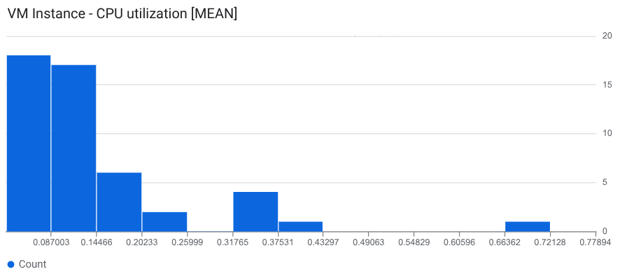
The example shows the most recent value for about 50 time series. The most
recent value for most of the time series is 0.145 or less.
To add a histogram to a dashboard, do the following:
1. [Open a dashboard and add a widget](https://docs.cloud.google.com/monitoring/charts#open).
2. In the widget menu, select **Histogram**.
3. [Select a metric type to display](https://docs.cloud.google.com/monitoring/charts#select-data).
A histogram is shown with a default bin configuration.
4. Optional: Update the bin configuration:
- To configure the number or size of the bins, select **Histogram bins**
and make a selection.
- To specify the number of bins, select **Count**, and then
enter a value. We recommend that the value you enter is at least
5 but not more than
50. However, this feature
supports up to 1000 bins.
- To specify the size of each bin, select **Size**, and then
enter a value.
- To specify the minimum and maximum x-axis values, select
**X-axis range** and complete the dialog.
- To specify linear or logarithmic scaling on the y-axis, select
**Y-axis scale** and complete the dialog.
5. Select **Apply** and then **Save**.
You can also use the Cloud Monitoring API to add a histogram widget to a
dashboard. For more information, see
[Dashboard with a `Histogram` widget](https://docs.cloud.google.com/monitoring/dashboards/api-examples#dashboard_with_a_histogram_widget).
### Configure a pie chart
To view the most recent data as a fraction of the total, add a pie chart.
Like tables, a pie chart can display any
[metric type](https://docs.cloud.google.com/monitoring/api/v3/metrics)
that has a numeric value, and it can display percentiles for
distribution-valued metrics. Each time series contributes
one slice to the pie.
The following screenshot illustrates a dashboard that displays
the CPU utilization of virtual machine instances by using two different
configurations of a **Pie chart** widget:

For information about how to add pie charts to a dashboard,
complete the following steps:
1. [Open a dashboard and add a widget](https://docs.cloud.google.com/monitoring/charts#open).
2. In the widget menu, select **Pie Chart**.
To display the total value, set the **Chart type** field to **Donut**.
3. [Select a metric type to display](https://docs.cloud.google.com/monitoring/charts#select-data).
For information about using the API to configure a pie chart, see
[Dashboard with a `PieChart` widget](https://docs.cloud.google.com/monitoring/dashboards/api-examples#dashboard_with_a_pie_widget).
### Configure a treemap
To view the most recent data as a nested series of rectangles, where each
rectangle corresponds to a unique collection of label values, add a treemap.
Assume that you've aggregated the data you are charting by the `zone` label.
If you set the widget type to treemap, then each rectangle on the
treemap corresponds to one zone. The color saturation of a rectangle is
proportional to the value it represents.
The following screenshot shows a treemap widget where the
time series are aggregated by `zone` and `storage_type`:
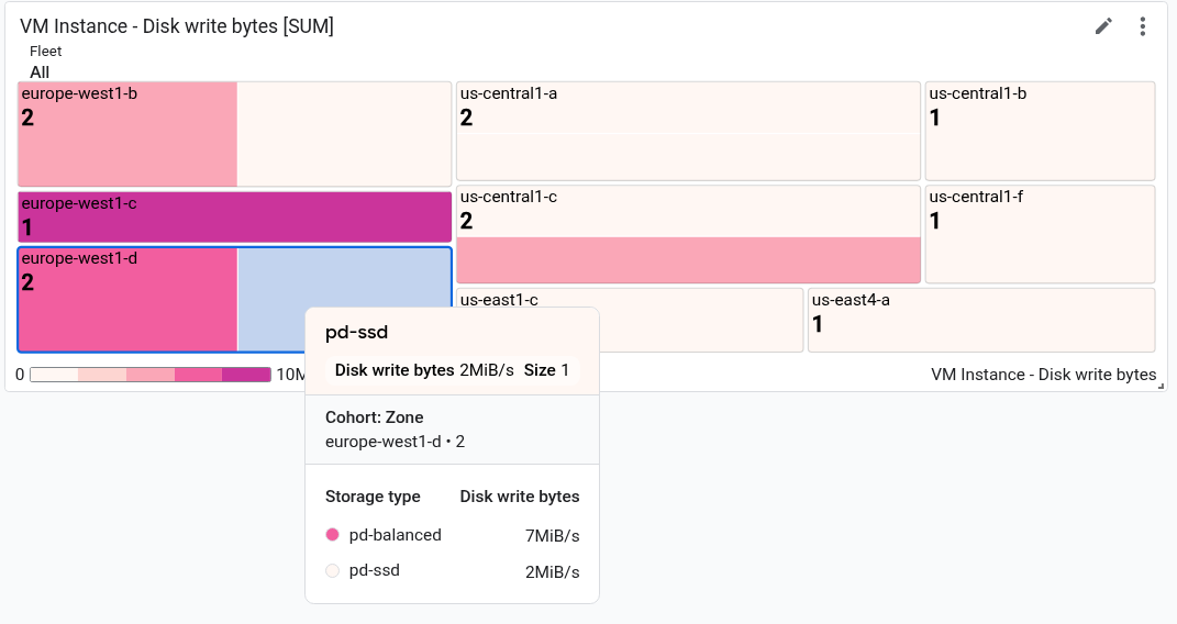
In the screenshot, the tooltip is shown for one rectangle.
To configure a treemap, do the following:
1. [Open a dashboard and add a widget](https://docs.cloud.google.com/monitoring/charts#open).
2. In the widget menu, select **Treemap**.
3. [Select a metric type to display](https://docs.cloud.google.com/monitoring/charts#select-data).
4. If the **Aggregation** element displays **Unaggregated** , then use the menu to select an aggregation function. For example, select **Mean** or **Max**.
5. In the second field of the **Aggregation** element, select at least one label.
6. To apply your changes to the dashboard, in the toolbar, click **Apply** . To discard your changes, click **Cancel**.
7. To save your modified dashboard, in the toolbar, click **Save**.
> [!NOTE]
> **Note:** If you want to change an existing widget to the treemap widget type, then ensure that you've aggregated the time series by at least one label.
For information about using the API to configure a treemap, see
[Dashboard with a `Treemap` widget](https://docs.cloud.google.com/monitoring/dashboards/api-examples#dashboard_with_a_treemap_widget).
## What's next
You can also add the following widgets to your custom dashboards:
- [Display alerts and charts for alerting policies](https://docs.cloud.google.com/monitoring/dashboards/alerts-and-incidents)
- [Log entries](https://docs.cloud.google.com/monitoring/charts/view-logs)
- [Descriptive text](https://docs.cloud.google.com/monitoring/dashboards/text-and-grouping)
- [Service-level objectives (SLOs) for a set of services](https://docs.cloud.google.com/monitoring/dashboards/slos)
For information about exploring charted data and filtering your dashboards,
see the following documents:
- [Explore charted data](https://docs.cloud.google.com/monitoring/charts/working-with-charts)
- [Add temporary filters to a custom dashboard](https://docs.cloud.google.com/monitoring/charts/filter-dashboard)
- [Create and manage variables and pinned filters](https://docs.cloud.google.com/monitoring/dashboards/filter-permanent)