This tutorial teaches you how to use an
[`ARIMA_PLUS` univariate time series model](https://docs.cloud.google.com/bigquery/docs/reference/standard-sql/bigqueryml-syntax-create-time-series.md.txt) to forecast the future value for a given column based on the historical values
for that column.
This tutorial forecasts a single time series. Forecasted values are
calculated once for each time point in the input data.
This tutorial uses data from the public
[`bigquery-public-data.google_analytics_sample.ga_sessions` sample table](https://console.cloud.google.com/bigquery?p=bigquery-public-data&d=google_analytics_sample&t=ga_sessions_20170801&page=table). This
table contains obfuscated ecommerce data from the Google Merchandise Store.
## Objectives
This tutorial guides you through completing the following tasks:
- Creating a time series model to forecast site traffic by using the [`CREATE MODEL` statement](https://docs.cloud.google.com/bigquery/docs/reference/standard-sql/bigqueryml-syntax-create-time-series.md.txt).
- Evaluating the autoregressive integrated moving average (ARIMA) information in the model by using the [`ML.ARIMA_EVALUATE` function](https://docs.cloud.google.com/bigquery/docs/reference/standard-sql/bigqueryml-syntax-arima-evaluate.md.txt).
- Inspecting the model coefficients by using the [`ML.ARIMA_COEFFICIENTS` function](https://docs.cloud.google.com/bigquery/docs/reference/standard-sql/bigqueryml-syntax-arima-coefficients.md.txt).
- Retrieving the forecasted site traffic information from the model by using the [`ML.FORECAST` function](https://docs.cloud.google.com/bigquery/docs/reference/standard-sql/bigqueryml-syntax-forecast.md.txt).
- Retrieving components of the time series, such as seasonality and trend, by using the [`ML.EXPLAIN_FORECAST` function](https://docs.cloud.google.com/bigquery/docs/reference/standard-sql/bigqueryml-syntax-explain-forecast.md.txt). You can inspect these time series components in order to explain the forecasted values.
## Costs
This tutorial uses billable components of Google Cloud, including the following:
- BigQuery
- BigQuery ML
For more information about BigQuery costs, see the
[BigQuery pricing](https://cloud.google.com/bigquery/pricing) page.
For more information about BigQuery ML costs, see
[BigQuery ML pricing](https://cloud.google.com/bigquery/pricing#bqml).
## Before you begin
1. BigQuery is automatically enabled in new projects. To activate BigQuery in a pre-existing project, go to
Enable the BigQuery API, if it is not already enabled.
**Roles required to enable APIs**
To enable APIs, you need the `serviceusage.services.enable` permission. If you
created the project, then you likely already have this permission through the
Owner role (`roles/owner`). Otherwise, you can get this permission through the
Service Usage Admin role (`roles/serviceusage.serviceUsageAdmin`).
[Learn how to grant roles](https://docs.cloud.google.com/iam/docs/granting-changing-revoking-access.md.txt).
[Enable the API](https://console.cloud.google.com/apis/enableflow?apiid=bigquery)
## Required Permissions
- To create the dataset, you need the `bigquery.datasets.create`
IAM permission.
- To create the model, you need the following permissions:
- `bigquery.jobs.create`
- `bigquery.models.create`
- `bigquery.models.getData`
- `bigquery.models.updateData`
- To run inference, you need the following permissions:
- `bigquery.models.getData`
- `bigquery.jobs.create`
For more information about IAM roles and permissions in
BigQuery, see
[Introduction to IAM](https://docs.cloud.google.com/bigquery/docs/access-control.md.txt).
## Create a dataset
To create a BigQuery dataset, select one of the following options:
### Console
1. In the Google Cloud console, go to the **BigQuery** page.
[Go to BigQuery](https://console.cloud.google.com/bigquery)
2. In the left pane, click
**Explorer**:

If you don't see the left pane, click
**Expand left pane** to open the pane.
3. In **Explorer** , expand your project, and then click **Datasets**.
4. On the **Datasets** page, click
**Create dataset**.
5. In the **Create dataset** pane, do the following:
- For **Dataset ID** , enter `bqml_tutorial`.
- For **Data location** , select **US**.
Leave the remaining default settings as they are.
6. Click **Create dataset**.
### bq
To create a new dataset, use the
[`bq mk --dataset` command](https://docs.cloud.google.com/bigquery/docs/reference/bq-cli-reference.md.txt#mk-dataset).
1. Create a dataset named `bqml_tutorial` with the data location set to `US`:
```
bq mk --dataset \
--location=US \
--description "BigQuery ML tutorial dataset." \
bqml_tutorial
```
2. Confirm that the dataset was created:
```bash
bq ls
```
### API
Call the [`datasets.insert`](https://docs.cloud.google.com/bigquery/docs/reference/rest/v2/datasets/insert.md.txt)
method with a defined [dataset resource](https://docs.cloud.google.com/bigquery/docs/reference/rest/v2/datasets.md.txt):
```json
{
"datasetReference": {
"datasetId": "bqml_tutorial"
}
}
```
### BigQuery DataFrames
Before trying this sample, follow the BigQuery DataFrames
setup instructions in the [BigQuery quickstart
using BigQuery DataFrames](https://docs.cloud.google.com/bigquery/docs/dataframes-quickstart).
For more information, see the
[BigQuery DataFrames reference documentation](https://docs.cloud.google.com/python/docs/reference/bigframes/latest.md.txt).
To authenticate to BigQuery, set up Application Default Credentials.
For more information, see [Set
up ADC for a local development environment](https://docs.cloud.google.com/docs/authentication/set-up-adc-local-dev-environment).
```python
import google.cloud.bigquery
bqclient = google.cloud.bigquery.Client()
bqclient.create_dataset("bqml_tutorial", exists_ok=True)
```
## Visualize the input data
Before creating the model, you can optionally visualize your input
time series data to get a sense of the distribution. You can do this by using Data Studio.
Follow these steps to visualize the time series data:
### SQL
In the following GoogleSQL query, the
`SELECT` statement parses the `date` column from the input
table to the `TIMESTAMP` type and renames it to `parsed_date`, and uses
the `SUM(...)` clause and the `GROUP BY date` clause to create a daily
`totals.visits` value.
1. In the Google Cloud console, go to the **BigQuery** page.
[Go to BigQuery](https://console.cloud.google.com/bigquery)
2. In the query editor, paste in the following query and click **Run**:
```googlesql
SELECT
PARSE_TIMESTAMP("%Y%m%d", date) AS parsed_date,
SUM(totals.visits) AS total_visits
FROM
`bigquery-public-data.google_analytics_sample.ga_sessions_*`
GROUP BY date;
```
1. When the query completes, click **Open in** \>
**Data Studio**. Data Studio opens in
a new tab. Complete the following steps in the new tab.
2. In Data Studio, click **Insert** \>
**Time series chart**.
3. In the **Chart** pane, choose the **Setup** tab.
4. In the **Metric** section, add the **total_visits** field, and remove the
default **Record Count** metric.
The resulting chart looks similar to the following:
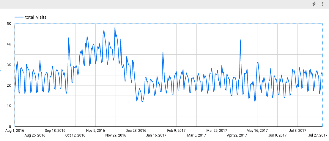
Looking at the chart, you can see that the input time series has a weekly seasonal pattern.
> [!NOTE]
> **Note:** For more information about Data Studio support, see [Data Studio help and support options](https://docs.cloud.google.com/looker/docs/studio/contact-us).
### BigQuery DataFrames
Before trying this sample, follow the BigQuery DataFrames
setup instructions in the [BigQuery quickstart
using BigQuery DataFrames](https://docs.cloud.google.com/bigquery/docs/dataframes-quickstart).
For more information, see the
[BigQuery DataFrames reference documentation](https://docs.cloud.google.com/python/docs/reference/bigframes/latest.md.txt).
To authenticate to BigQuery, set up Application Default Credentials.
For more information, see [Set
up ADC for a local development environment](https://docs.cloud.google.com/docs/authentication/set-up-adc-local-dev-environment).
```python
import bigframes.pandas as bpd
# Set partial ordering mode for BigQuery DataFrames.
# For more information, see the BigQuery DataFrames performance documentation:
# https://cloud.google.com/bigquery/docs/dataframes-performance#partial-ordering-mode
bpd.options.bigquery.ordering_mode = "partial"
# Start by loading the historical data from BigQuerythat you want to analyze and forecast.
# This clause indicates that you are querying the ga_sessions_* tables in the google_analytics_sample dataset.
# Read and visualize the time series you want to forecast.
df = bpd.read_gbq("bigquery-public-data.google_analytics_sample.ga_sessions_*")
parsed_date = bpd.to_datetime(df.date, format="%Y%m%d", utc=True)
parsed_date.name = "parsed_date"
visits = df["totals"].struct.field("visits")
visits.name = "total_visits"
total_visits = visits.groupby(parsed_date).sum()
# Expected output: total_visits.head()
# parsed_date
# 2016-08-01 00:00:00+00:00 1711
# 2016-08-02 00:00:00+00:00 2140
# 2016-08-03 00:00:00+00:00 2890
# 2016-08-04 00:00:00+00:00 3161
# 2016-08-05 00:00:00+00:00 2702
# Name: total_visits, dtype: Int64
total_visits.plot.line()
```
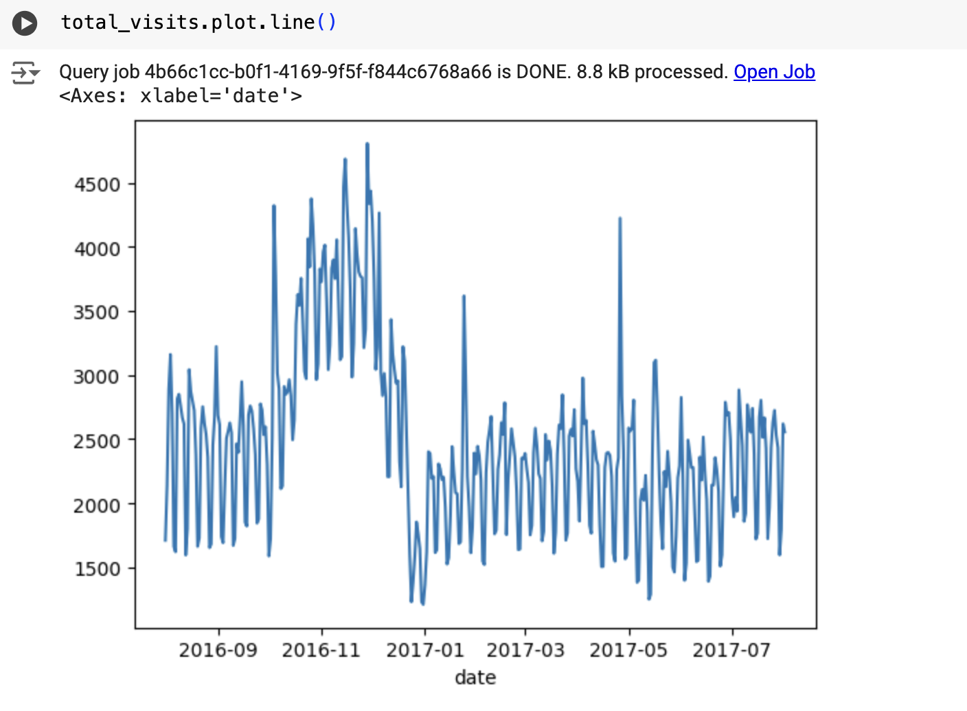
The result is similar to the following:
## Create the time series model
Create a time series model to forecast total site visits as represented by
`totals.visits` column, and train it on the Google Analytics 360
data.
### SQL
In the following query, the
`OPTIONS(model_type='ARIMA_PLUS', time_series_timestamp_col='date', ...)`
clause indicates that you are creating an
[ARIMA](https://en.wikipedia.org/wiki/Autoregressive_integrated_moving_average)-based
time series model. The
[`auto_arima` option](https://docs.cloud.google.com/bigquery/docs/reference/standard-sql/bigqueryml-syntax-create-multivariate-time-series.md.txt#auto_arima)
of the `CREATE MODEL` statement defaults to `TRUE`, so the `auto.ARIMA`
algorithm automatically tunes the hyperparameters in the model. The algorithm
fits dozens of candidate models and chooses the best model, which is the model
with the lowest
[Akaike information criterion (AIC)](https://en.wikipedia.org/wiki/Akaike_information_criterion).
The
[`data_frequency` option](https://docs.cloud.google.com/bigquery/docs/reference/standard-sql/bigqueryml-syntax-create-multivariate-time-series.md.txt#data_frequency)
of the `CREATE MODEL` statements defaults to `AUTO_FREQUENCY`, so the
training process automatically infers the data frequency of the input time
series. The
[`decompose_time_series` option](https://docs.cloud.google.com/bigquery/docs/reference/standard-sql/bigqueryml-syntax-create-time-series.md.txt#decompose_time_series)
of the `CREATE MODEL` statement defaults to `TRUE`, so that information about
the time series data is returned when you evaluate the model in the next step.
Follow these steps to create the model:
1. In the Google Cloud console, go to the **BigQuery** page.
[Go to BigQuery](https://console.cloud.google.com/bigquery)
2. In the query editor, paste in the following query and click **Run**:
```googlesql
CREATE OR REPLACE MODEL `bqml_tutorial.ga_arima_model`
OPTIONS
(model_type = 'ARIMA_PLUS',
time_series_timestamp_col = 'parsed_date',
time_series_data_col = 'total_visits',
auto_arima = TRUE,
data_frequency = 'AUTO_FREQUENCY',
decompose_time_series = TRUE
) AS
SELECT
PARSE_TIMESTAMP("%Y%m%d", date) AS parsed_date,
SUM(totals.visits) AS total_visits
FROM
`bigquery-public-data.google_analytics_sample.ga_sessions_*`
GROUP BY date;
```
The query takes about 4 seconds to complete, after which you can access the
`ga_arima_model` model. Because the query uses a `CREATE MODEL` statement
to create a model, you don't see query results.
> [!NOTE]
> **Note:** You might wonder if United States holidays have an impact on the time series. You can try setting the [`holiday_region` option](https://docs.cloud.google.com/bigquery/docs/reference/standard-sql/bigqueryml-syntax-create-multivariate-time-series.md.txt#holiday_region) of the `CREATE MODEL` statement to `US`. Setting this option allows a more accurate modeling on holiday time points if there are any holiday patterns in the time series.
### BigQuery DataFrames
Before trying this sample, follow the BigQuery DataFrames
setup instructions in the [BigQuery quickstart
using BigQuery DataFrames](https://docs.cloud.google.com/bigquery/docs/dataframes-quickstart).
For more information, see the
[BigQuery DataFrames reference documentation](https://docs.cloud.google.com/python/docs/reference/bigframes/latest.md.txt).
To authenticate to BigQuery, set up Application Default Credentials.
For more information, see [Set
up ADC for a local development environment](https://docs.cloud.google.com/docs/authentication/set-up-adc-local-dev-environment).
```python
import bigframes.pandas as bpd
from bigframes.bigquery import ml
# Set partial ordering mode for BigQuery DataFrames.
# For more information, see the BigQuery DataFrames performance documentation:
# https://cloud.google.com/bigquery/docs/dataframes-performance#partial-ordering-mode
bpd.options.bigquery.ordering_mode = "partial"
# Use the data loaded in the previous step to fit the model
training_data = total_visits.to_frame().reset_index(drop=False)
# Create a time series model to forecast total site visits:
# The auto_arima option defaults to True, so the auto.ARIMA algorithm automatically
# tunes the hyperparameters in the model.
# The data_frequency option defaults to 'auto_frequency so the training
# process automatically infers the data frequency of the input time series.
# The decompose_time_series option defaults to True, so that information about
# the time series data is returned when you evaluate the model in the next step.
# For more information, see the BigQuery DataFrames API reference documentation:
# https://dataframes.bigquery.dev/reference/api/bigframes.bigquery.ml.create_model.html#bigframes.bigquery.ml.create_model
ml.create_model(
your_model_id, # For example: "bqml_tutorial.ga_arima_model"
options={
"model_type": "ARIMA_PLUS",
"time_series_timestamp_col": "parsed_date",
"time_series_data_col": "total_visits",
"auto_arima": True,
"data_frequency": "AUTO_FREQUENCY",
"decompose_time_series": True,
},
training_data=training_data,
replace=True,
)
```
## Evaluate the candidate models
### SQL
Evaluate the time series models by using the `ML.ARIMA_EVALUATE`
function. The `ML.ARIMA_EVALUATE` function shows you the evaluation metrics of
all the candidate models evaluated during the process of automatic
hyperparameter tuning.
Follow these steps to evaluate the model:
1. In the Google Cloud console, go to the **BigQuery** page.
[Go to BigQuery](https://console.cloud.google.com/bigquery)
2. In the query editor, paste in the following query and click **Run**:
```googlesql
SELECT
*
FROM
ML.ARIMA_EVALUATE(MODEL `bqml_tutorial.ga_arima_model`);
```
The results should look similar to the following:

### BigQuery DataFrames
Before trying this sample, follow the BigQuery DataFrames
setup instructions in the [BigQuery quickstart
using BigQuery DataFrames](https://docs.cloud.google.com/bigquery/docs/dataframes-quickstart).
For more information, see the
[BigQuery DataFrames reference documentation](https://docs.cloud.google.com/python/docs/reference/bigframes/latest.md.txt).
To authenticate to BigQuery, set up Application Default Credentials.
For more information, see [Set
up ADC for a local development environment](https://docs.cloud.google.com/docs/authentication/set-up-adc-local-dev-environment).
```python
import bigframes.pandas as bpd
from bigframes.bigquery import ml
# Set partial ordering mode for BigQuery DataFrames.
# For more information, see the BigQuery DataFrames performance documentation:
# https://cloud.google.com/bigquery/docs/dataframes-performance#partial-ordering-mode
bpd.options.bigquery.ordering_mode = "partial"
# For more information, see the BigQuery DataFrames API reference documentation:
# https://dataframes.bigquery.dev/reference/api/bigframes.bigquery.ml.arima_evaluate.html#bigframes.bigquery.ml.arima_evaluate
ml.arima_evaluate(
your_model_id, # For example: "bqml_tutorial.ga_arima_model"
show_all_candidate_models=True,
)
# Expected output:
# row non_seasonal_p non_seasonal_d non_seasonal_q has_drift log_likelihood AIC variance seasonal_periods has_holiday_effect has_spikes_and_dips has_step_changes error_message
# 0 0 1 3 True -2464.255656 4938.511313 42772.506055 ['WEEKLY'] False False True
# 1 2 1 0 False -2473.141651 4952.283303 44942.416463 ['WEEKLY'] False False True
# 2 1 1 0 False -2479.880885 4963.76177 46642.953433 ['WEEKLY'] False False True
# 3 0 1 1 False -2470.632377 4945.264753 44319.379307 ['WEEKLY'] False False True
# 4 2 1 1 True -2463.671247 4937.342493 42633.299513 ['WEEKLY'] False False True
```
The `non_seasonal_p`, `non_seasonal_d`, `non_seasonal_q`, and `has_drift`
output columns define an ARIMA model in the training pipeline. The
`log_likelihood`, `AIC`, and `variance` output columns are relevant to the ARIMA
model fitting process.
The `auto.ARIMA` algorithm uses the
[KPSS test](https://en.wikipedia.org/wiki/KPSS_test) to determine the best value
for `non_seasonal_d`, which in this case is `1`. When `non_seasonal_d` is `1`,
the `auto.ARIMA` algorithm trains 42 different candidate ARIMA models in parallel.
In this example, all 42 candidate models are valid, so the output contains 42
rows, one for each candidate ARIMA model; in cases where some of the models
aren't valid, they are excluded from the output. These candidate models are
returned in ascending order by AIC. The model in the first row has the lowest
AIC, and is considered the best model. The best model is saved as the final
model and is used when you call functions such as `ML.FORECAST` on the model
The `seasonal_periods` column contains information about the seasonal pattern
identified in the time series data. It has nothing to do with the ARIMA
modeling, therefore it has the same value across all output rows. It reports a
weekly pattern, which agrees with the results you saw if you chose to
visualize the input data.
The `has_holiday_effect`, `has_spikes_and_dips`, and `has_step_changes` columns
are only populated when `decompose_time_series=TRUE`. These columns also reflect
information about the input time series data, and are not related to the ARIMA
modeling. These columns also have the same values across all output rows.
The `error_message` column shows any errors that incurred during the
`auto.ARIMA` fitting process. One possible reason for errors is when the selected
`non_seasonal_p`, `non_seasonal_d`, `non_seasonal_q`, and `has_drift` columns
are not able to stabilize the time series. To retrieve the error
message of all the candidate models, set the `show_all_candidate_models`
argument of the `ML.ARIMA_EVALUATE` function to `TRUE`. For single time series
models, `TRUE` is the default.
For more information about the output columns, see
[`ML.ARIMA_EVALUATE` function](https://docs.cloud.google.com/bigquery/docs/reference/standard-sql/bigqueryml-syntax-arima-evaluate.md.txt).
## Inspect the model's coefficients
### SQL
Inspect the time series model's coefficients by using the
`ML.ARIMA_COEFFICIENTS` function.
Follow these steps to retrieve the model's coefficients:
1. In the Google Cloud console, go to the **BigQuery** page.
[Go to BigQuery](https://console.cloud.google.com/bigquery)
2. In the query editor, paste in the following query and click **Run**:
```googlesql
SELECT
*
FROM
ML.ARIMA_COEFFICIENTS(MODEL `bqml_tutorial.ga_arima_model`);
```
The `ar_coefficients` output column shows the model coefficients of the
autoregressive (AR) part of the ARIMA model. Similarly, the `ma_coefficients`
output column shows the model coefficients of the moving-average (MA) part of
the ARIMA model. Both of these columns contain array values, whose lengths are
equal to `non_seasonal_p` and `non_seasonal_q`, respectively. You saw in the
output of the `ML.ARIMA_EVALUATE` function that the best model has a
`non_seasonal_p` value of `2` and a `non_seasonal_q` value of `3`. Therefore, in
the `ML.ARIMA_COEFFICIENTS` output, the `ar_coefficients` value is a 2-element
array and the `ma_coefficients` value is a 3-element array. The
`intercept_or_drift` value is the constant term in the ARIMA model.
For more information about the output columns, see
[`ML.ARIMA_COEFFICIENTS` function](https://docs.cloud.google.com/bigquery/docs/reference/standard-sql/bigqueryml-syntax-arima-coefficients.md.txt).
### BigQuery DataFrames
Inspect the time series model's coefficients by using the
[`bigframes.bigquery.ml.arima_coefficients` function](https://dataframes.bigquery.dev/reference/api/bigframes.bigquery.ml.arima_coefficients.html#bigframes.bigquery.ml.arima_coefficients).
Before trying this sample, follow the BigQuery DataFrames
setup instructions in the [BigQuery quickstart
using BigQuery DataFrames](https://docs.cloud.google.com/bigquery/docs/dataframes-quickstart).
For more information, see the
[BigQuery DataFrames reference documentation](https://docs.cloud.google.com/python/docs/reference/bigframes/latest.md.txt).
To authenticate to BigQuery, set up Application Default Credentials.
For more information, see [Set
up ADC for a local development environment](https://docs.cloud.google.com/docs/authentication/set-up-adc-local-dev-environment).
```python
import bigframes.pandas as bpd
from bigframes.bigquery import ml
# Set partial ordering mode for BigQuery DataFrames.
# For more information, see the BigQuery DataFrames performance documentation:
# https://cloud.google.com/bigquery/docs/dataframes-performance#partial-ordering-mode
bpd.options.bigquery.ordering_mode = "partial"
# For more information, see the BigQuery DataFrames API reference documentation:
# https://dataframes.bigquery.dev/reference/api/bigframes.bigquery.ml.arima_coefficients.html#bigframes.bigquery.ml.arima_coefficients
ml.arima_coefficients(
your_model_id, # For example: "bqml_tutorial.ga_arima_model"
)
# Expected output:
# ar_coefficients ma_coefficients intercept_or_drift
# 0 [0.40944762] [-0.81168198] 0.0
```
The `ar_coefficients` output column shows the model coefficients of the
autoregressive (AR) part of the ARIMA model. Similarly, the `ma_coefficients`
output column shows the model coefficients of the moving-average (MA) part of
the ARIMA model. Both of these columns contain array values, whose lengths are
equal to `non_seasonal_p` and `non_seasonal_q`, respectively.
## Use the model to forecast data
### SQL
Forecast future time series values by using the `ML.FORECAST`
function.
In the following GoogleSQL query, the
`STRUCT(30 AS horizon, 0.8 AS confidence_level)` clause indicates that the
query forecasts 30 future time points, and generates a prediction interval
with an 80% confidence level.
Follow these steps to forecast data with the model:
1. In the Google Cloud console, go to the **BigQuery** page.
[Go to BigQuery](https://console.cloud.google.com/bigquery)
2. In the query editor, paste in the following query and click **Run**:
```googlesql
SELECT
*
FROM
ML.FORECAST(MODEL `bqml_tutorial.ga_arima_model`,
STRUCT(30 AS horizon, 0.8 AS confidence_level));
```
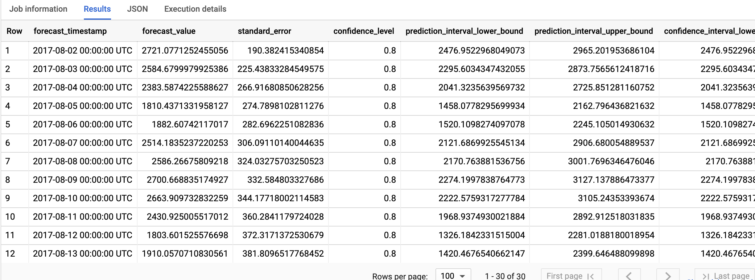
The results should look similar to the following:
### BigQuery DataFrames
Forecast future time series values by using the
[`bigframes.bigquery.ml.forecast` function](https://dataframes.bigquery.dev/reference/api/bigframes.bigquery.ml.forecast.html#bigframes.bigquery.ml.forecast).
Before trying this sample, follow the BigQuery DataFrames
setup instructions in the [BigQuery quickstart
using BigQuery DataFrames](https://docs.cloud.google.com/bigquery/docs/dataframes-quickstart).
For more information, see the
[BigQuery DataFrames reference documentation](https://docs.cloud.google.com/python/docs/reference/bigframes/latest.md.txt).
To authenticate to BigQuery, set up Application Default Credentials.
For more information, see [Set
up ADC for a local development environment](https://docs.cloud.google.com/docs/authentication/set-up-adc-local-dev-environment).
```python
import bigframes.pandas as bpd
from bigframes.bigquery import ml
# Set partial ordering mode for BigQuery DataFrames.
# For more information, see the BigQuery DataFrames performance documentation:
# https://cloud.google.com/bigquery/docs/dataframes-performance#partial-ordering-mode
bpd.options.bigquery.ordering_mode = "partial"
# For more information, see the BigQuery DataFrames API reference documentation:
# https://dataframes.bigquery.dev/reference/api/bigframes.bigquery.ml.forecast.html#bigframes.bigquery.ml.forecast
ml.forecast(
your_model_id, # For example: "bqml_tutorial.ga_arima_model"
horizon=30,
confidence_level=0.8,
)
# Expected output:
# forecast_timestamp forecast_value standard_error confidence_level prediction_interval_lower_bound prediction_interval_upper_bound confidence_interval_lower_bound confidence_interval_upper_bound
# 11 2017-08-13 00:00:00+00:00 1845.439732 328.060405 0.8 1424.772257 2266.107208 1424.772257 2266.107208
# 29 2017-08-31 00:00:00+00:00 2615.993932 431.286628 0.8 2062.960849 3169.027015 2062.960849 3169.027015
# 7 2017-08-09 00:00:00+00:00 2639.285993 300.301186 0.8 2254.213792 3024.358193 2254.213792 3024.358193
# 25 2017-08-27 00:00:00+00:00 1853.735689 410.596551 0.8 1327.233216 2380.238162 1327.233216 2380.238162
# 1 2017-08-03 00:00:00+00:00 2621.33159 241.093355 0.8 2312.180802 2930.482379 2312.180802 2930.482379
```
The output rows are in chronological order by the
`forecast_timestamp` column value. In time series forecasting, the prediction
interval, as represented by the `prediction_interval_lower_bound` and
`prediction_interval_upper_bound` column values, is as important as the
`forecast_value` column value. The `forecast_value` value is the middle point
of the prediction interval. The prediction interval depends on the
`standard_error` and `confidence_level` column values.
For more information about the output columns, see
[`ML.FORECAST` function](https://docs.cloud.google.com/bigquery/docs/reference/standard-sql/bigqueryml-syntax-forecast.md.txt).
## Explain the forecasting results
### SQL
You can get explainability metrics in addition to forecast data by using the
`ML.EXPLAIN_FORECAST` function. The `ML.EXPLAIN_FORECAST` function forecasts
future time series values and also returns all the separate components of the
time series.
Similar to the `ML.FORECAST` function, the
`STRUCT(30 AS horizon, 0.8 AS confidence_level)` clause used in the
`ML.EXPLAIN_FORECAST` function indicates that the query forecasts 30 future
time points and generates a prediction interval with 80% confidence.
Follow these steps to explain the model's results:
1. In the Google Cloud console, go to the **BigQuery** page.
[Go to BigQuery](https://console.cloud.google.com/bigquery)
2. In the query editor, paste in the following query and click **Run**:
```googlesql
SELECT
*
FROM
ML.EXPLAIN_FORECAST(MODEL `bqml_tutorial.ga_arima_model`,
STRUCT(30 AS horizon, 0.8 AS confidence_level));
```
The results should look similar to the following:
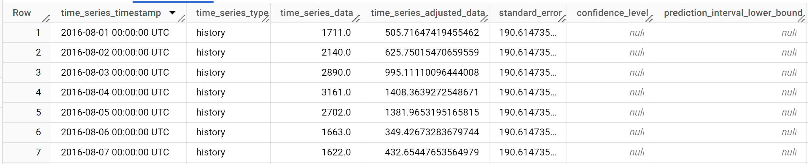
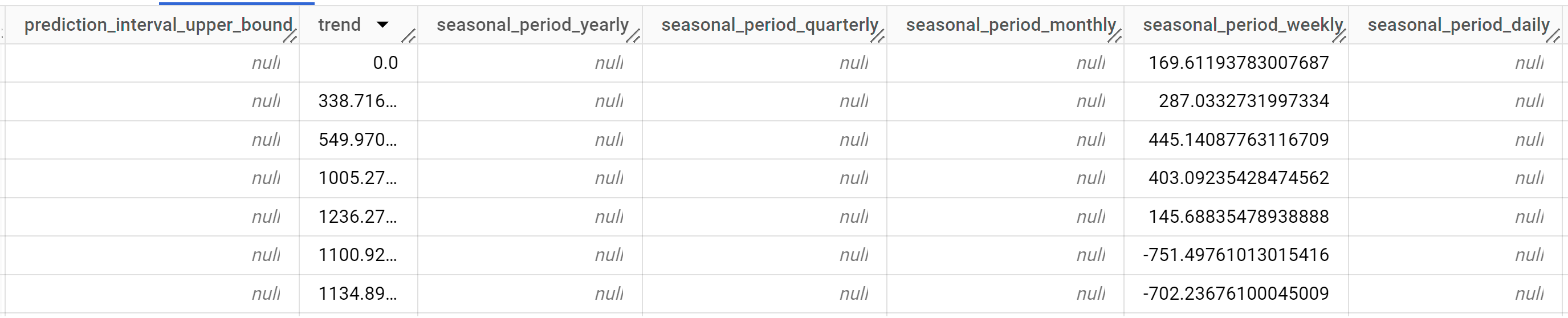
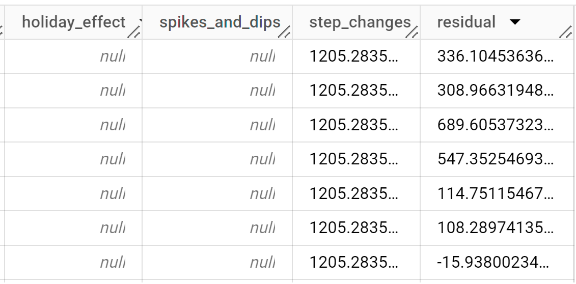
The output rows are ordered chronologically by the `time_series_timestamp`
column value.
For more information about the output columns, see
[`ML.EXPLAIN_FORECAST` function](https://docs.cloud.google.com/bigquery/docs/reference/standard-sql/bigqueryml-syntax-explain-forecast.md.txt).
### BigQuery DataFrames
You can get explainability metrics in addition to forecast data by using the
[`bigframes.bigquery.ml.explain_forecast` function](https://dataframes.bigquery.dev/reference/api/bigframes.bigquery.ml.explain_forecast.html#bigframes.bigquery.ml.explain_forecast).
The `bigframes.bigquery.ml.explain_forecast` function forecasts
future time series values and also returns all the separate components of the
time series.
Similar to the `bigframes.bigquery.ml.forecast` function, the
`horizon=30, confidence_level=0.8` arguments used in the
`bigframes.bigquery.ml.explain_forecast` function indicate that the query
forecasts 30 future time points and generates a prediction interval with
80% confidence.
Before trying this sample, follow the BigQuery DataFrames
setup instructions in the [BigQuery quickstart
using BigQuery DataFrames](https://docs.cloud.google.com/bigquery/docs/dataframes-quickstart).
For more information, see the
[BigQuery DataFrames reference documentation](https://docs.cloud.google.com/python/docs/reference/bigframes/latest.md.txt).
To authenticate to BigQuery, set up Application Default Credentials.
For more information, see [Set
up ADC for a local development environment](https://docs.cloud.google.com/docs/authentication/set-up-adc-local-dev-environment).
```python
import bigframes.pandas as bpd
from bigframes.bigquery import ml
# Set partial ordering mode for BigQuery DataFrames.
# For more information, see the BigQuery DataFrames performance documentation:
# https://cloud.google.com/bigquery/docs/dataframes-performance#partial-ordering-mode
bpd.options.bigquery.ordering_mode = "partial"
# For more information, see the BigQuery DataFrames API reference documentation:
# https://dataframes.bigquery.dev/reference/api/bigframes.bigquery.ml.explain_forecast.html#bigframes.bigquery.ml.explain_forecast
ml.explain_forecast(
your_model_id, # For example: "bqml_tutorial.ga_arima_model"
horizon=30,
confidence_level=0.8,
)
# Expected output:
# time_series_timestamp time_series_type time_series_data time_series_adjusted_data standard_error confidence_level prediction_interval_lower_bound prediction_interval_upper_bound trend seasonal_period_yearly seasonal_period_quarterly seasonal_period_monthly seasonal_period_weekly seasonal_period_daily holiday_effect spikes_and_dips step_changes residual
# 0 2016-08-01 00:00:00+00:00 history 1711.0 505.716474 206.939556 0.0 169.611938 1205.283526 336.104536
# 1 2016-08-02 00:00:00+00:00 history 2140.0 623.137701 206.939556 336.104428 287.033273 1205.283526 311.578773
# 2 2016-08-03 00:00:00+00:00 history 2890.0 1008.655091 206.939556 563.514213 445.140878 1205.283526 676.061383
# 3 2016-08-04 00:00:00+00:00 history 3161.0 1389.40959 206.939556 986.317236 403.092354 1205.283526 566.306884
# 4 2016-08-05 00:00:00+00:00 history 2702.0 1394.395741 206.939556 1248.707386 145.688355 1205.283526 102.320733
# 5 2016-08-06 00:00:00+00:00 history 1663.0 437.09243 206.939556 1188.59004 -751.49761 1205.283526 20.624044
```
If you would like to visualize the results, you can use
Data Studio as described in the
[Visualize the input data](https://docs.cloud.google.com/bigquery/docs/arima-single-time-series-forecasting-tutorial.md.txt#visualize_the_input_data)
section to create a chart, using the following columns as metrics:
- `time_series_data`
- `prediction_interval_lower_bound`
- `prediction_interval_upper_bound`
- `trend`
- `seasonal_period_weekly`
- `step_changes`
## Clean up
To avoid incurring charges to your Google Cloud account for the resources used in this
tutorial, either delete the project that contains the resources, or keep the project and
delete the individual resources.
- You can delete the project you created.
- Or you can keep the project and delete the dataset.
### Delete your dataset
Deleting your project removes all datasets and all tables in the project. If you
prefer to reuse the project, you can delete the dataset you created in this
tutorial:
1. If necessary, open the BigQuery page in the
Google Cloud console.
[Go to the BigQuery page](https://console.cloud.google.com/bigquery)
2. In the navigation, click the **bqml_tutorial** dataset you created.
3. Click **Delete dataset** on the right side of the window.
This action deletes the dataset, the table, and all the data.
4. In the **Delete dataset** dialog box, confirm the delete command by typing
the name of your dataset (`bqml_tutorial`) and then click **Delete**.
### Delete your project
To delete the project:
> [!CAUTION]
> **Caution** : Deleting a project has the following effects:
>
> - **Everything in the project is deleted.** If you used an existing project for the tasks in this document, when you delete it, you also delete any other work you've done in the project.
> - **Custom project IDs are lost.** When you created this project, you might have created a custom project ID that you want to use in the future. To preserve the URLs that use the project ID, such as an `appspot.com` URL, delete selected resources inside the project instead of deleting the whole project.
>
>
> If you plan to explore multiple architectures, tutorials, or quickstarts, reusing projects
> can help you avoid exceeding project quota limits.
1. In the Google Cloud console, go to the **Manage resources** page.
[Go to Manage resources](https://console.cloud.google.com/iam-admin/projects)
2. In the project list, select the project that you want to delete, and then click **Delete**.
3. In the dialog, type the project ID, and then click **Shut down** to delete the project.
## What's next
- Learn how to [forecast a single time series with a multivariate model](https://docs.cloud.google.com/bigquery/docs/arima-plus-xreg-single-time-series-forecasting-tutorial.md.txt)
- Learn how to [forecast multiple time series with a univariate model](https://docs.cloud.google.com/bigquery/docs/arima-multiple-time-series-forecasting-tutorial.md.txt)
- Learn how to [scale a univariate model when forecasting multiple time series over many rows](https://docs.cloud.google.com/bigquery/docs/arima-speed-up-tutorial.md.txt).
- Learn how to [hierarchically forecast multiple time series with a univariate model](https://docs.cloud.google.com/bigquery/docs/arima-time-series-forecasting-with-hierarchical-time-series.md.txt)
- For an overview of BigQuery ML, see [Introduction to AI and ML in BigQuery](https://docs.cloud.google.com/bigquery/docs/bqml-introduction.md.txt).