This tutorial teaches you how to use an
[`ARIMA_PLUS` univariate time series model](https://docs.cloud.google.com/bigquery/docs/reference/standard-sql/bigqueryml-syntax-create-time-series.md.txt) to forecast the future value of a given
column, based on the historical values for that column.
This tutorial forecasts for multiple time series. Forecasted values are
calculated for each time point, for each value in one or more specified columns.
For example, if you wanted to forecast weather and specified a column containing
city data, the forecasted data would contain forecasts for all time points for
City A, then forecasted values for all time points for City B, and so forth.
This tutorial uses data from the public
[`bigquery-public-data.new_york.citibike_trips`](https://console.cloud.google.com/bigquery?p=bigquery-public-data&d=new_york&t=citibike_trips&page=table)
table. This table contains information about Citi Bike trips in New York City.
Before reading this tutorial, we highly recommend that you read
[Forecast a single time series with a univariate model](https://docs.cloud.google.com/bigquery/docs/arima-single-time-series-forecasting-tutorial.md.txt).
## Objectives
This tutorial guides you through completing the following tasks:
- Creating a time series model to forecast the number of bike trips by using the [`CREATE MODEL` statement](https://docs.cloud.google.com/bigquery/docs/reference/standard-sql/bigqueryml-syntax-create-time-series.md.txt).
- Evaluating the autoregressive integrated moving average (ARIMA) information in the model by using the [`ML.ARIMA_EVALUATE` function](https://docs.cloud.google.com/bigquery/docs/reference/standard-sql/bigqueryml-syntax-arima-evaluate.md.txt).
- Inspecting the model coefficients by using the [`ML.ARIMA_COEFFICIENTS` function](https://docs.cloud.google.com/bigquery/docs/reference/standard-sql/bigqueryml-syntax-arima-coefficients.md.txt).
- Retrieving the forecasted bike ride information from the model by using the [`ML.FORECAST` function](https://docs.cloud.google.com/bigquery/docs/reference/standard-sql/bigqueryml-syntax-forecast.md.txt).
- Retrieving components of the time series, such as seasonality and trend, by using the [`ML.EXPLAIN_FORECAST` function](https://docs.cloud.google.com/bigquery/docs/reference/standard-sql/bigqueryml-syntax-explain-forecast.md.txt). You can inspect these time series components in order to explain the forecasted values.
## Costs
This tutorial uses billable components of Google Cloud, including:
- BigQuery
- BigQuery ML
For more information about BigQuery costs, see the
[BigQuery pricing](https://cloud.google.com/bigquery/pricing) page.
For more information about BigQuery ML costs, see
[BigQuery ML pricing](https://cloud.google.com/bigquery/pricing#bqml).
## Before you begin
1. BigQuery is automatically enabled in new projects. To activate BigQuery in a pre-existing project, go to
Enable the BigQuery API, if it is not already enabled.
**Roles required to enable APIs**
To enable APIs, you need the `serviceusage.services.enable` permission. If you
created the project, then you likely already have this permission through the
Owner role (`roles/owner`). Otherwise, you can get this permission through the
Service Usage Admin role (`roles/serviceusage.serviceUsageAdmin`).
[Learn how to grant roles](https://docs.cloud.google.com/iam/docs/granting-changing-revoking-access.md.txt).
[Enable the API](https://console.cloud.google.com/apis/enableflow?apiid=bigquery)
## Required Permissions
- To create the dataset, you need the `bigquery.datasets.create`
IAM permission.
- To create the model, you need the following permissions:
- `bigquery.jobs.create`
- `bigquery.models.create`
- `bigquery.models.getData`
- `bigquery.models.updateData`
- To run inference, you need the following permissions:
- `bigquery.models.getData`
- `bigquery.jobs.create`
For more information about IAM roles and permissions in
BigQuery, see
[Introduction to IAM](https://docs.cloud.google.com/bigquery/docs/access-control.md.txt).
## Create a dataset
To create a BigQuery dataset, select one of the following options:
### Console
1. In the Google Cloud console, go to the **BigQuery** page.
[Go to BigQuery](https://console.cloud.google.com/bigquery)
2. In the left pane, click
**Explorer**:

If you don't see the left pane, click
**Expand left pane** to open the pane.
3. In **Explorer** , expand your project, and then click **Datasets**.
4. On the **Datasets** page, click
**Create dataset**.
5. In the **Create dataset** pane, do the following:
- For **Dataset ID** , enter `bqml_tutorial`.
- For **Data location** , select **US**.
Leave the remaining default settings as they are.
6. Click **Create dataset**.
### bq
To create a new dataset, use the
[`bq mk --dataset` command](https://docs.cloud.google.com/bigquery/docs/reference/bq-cli-reference.md.txt#mk-dataset).
1. Create a dataset named `bqml_tutorial` with the data location set to `US`:
```
bq mk --dataset \
--location=US \
--description "BigQuery ML tutorial dataset." \
bqml_tutorial
```
2. Confirm that the dataset was created:
```bash
bq ls
```
### API
Call the [`datasets.insert`](https://docs.cloud.google.com/bigquery/docs/reference/rest/v2/datasets/insert.md.txt)
method with a defined [dataset resource](https://docs.cloud.google.com/bigquery/docs/reference/rest/v2/datasets.md.txt):
```json
{
"datasetReference": {
"datasetId": "bqml_tutorial"
}
}
```
### BigQuery DataFrames
Before trying this sample, follow the BigQuery DataFrames
setup instructions in the [BigQuery quickstart
using BigQuery DataFrames](https://docs.cloud.google.com/bigquery/docs/dataframes-quickstart).
For more information, see the
[BigQuery DataFrames reference documentation](https://docs.cloud.google.com/python/docs/reference/bigframes/latest.md.txt).
To authenticate to BigQuery, set up Application Default Credentials.
For more information, see [Set
up ADC for a local development environment](https://docs.cloud.google.com/docs/authentication/set-up-adc-local-dev-environment).
```python
import google.cloud.bigquery
bqclient = google.cloud.bigquery.Client()
bqclient.create_dataset("bqml_tutorial", exists_ok=True)
```
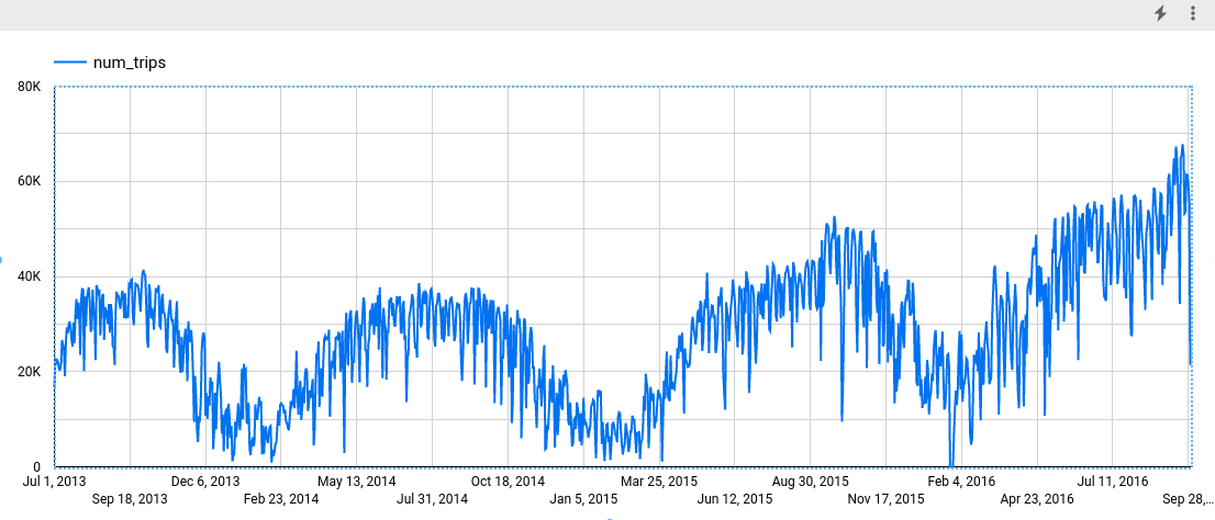
## Visualize the input data
Before creating the model, you can optionally visualize your input
time series data to get a sense of the distribution. You can do this by using
Data Studio.
### SQL
The `SELECT` statement of the following query uses the
[`EXTRACT` function](https://docs.cloud.google.com/bigquery/docs/reference/standard-sql/timestamp_functions.md.txt#extract)
to extract the date information from the `starttime` column. The query uses
the `COUNT(*)` clause to get the daily total number of Citi Bike trips.
Follow these steps to visualize the time series data:
1. In the Google Cloud console, go to the **BigQuery** page.
[Go to BigQuery](https://console.cloud.google.com/bigquery)
2. In the query editor, paste in the following query and click **Run**:
```googlesql
SELECT
EXTRACT(DATE from starttime) AS date,
COUNT(*) AS num_trips
FROM
`bigquery-public-data.new_york.citibike_trips`
GROUP BY date;
```
3. When the query completes, click **Open in** \>
**Data Studio**. Data Studio opens in
a new tab. Complete the following steps in the new tab.
4. In Data Studio, click **Insert** \>
**Time series chart**.
5. In the **Chart** pane, choose the **Setup** tab.
6. In the **Metric** section, add the **num_trips** field,
and remove the default **Record Count** metric.
The resulting chart looks similar to the following:
### BigQuery DataFrames
Before trying this sample, follow the BigQuery DataFrames
setup instructions in the [BigQuery quickstart
using BigQuery DataFrames](https://docs.cloud.google.com/bigquery/docs/dataframes-quickstart).
For more information, see the
[BigQuery DataFrames reference documentation](https://docs.cloud.google.com/python/docs/reference/bigframes/latest.md.txt).
To authenticate to BigQuery, set up Application Default Credentials.
For more information, see [Set
up ADC for a local development environment](https://docs.cloud.google.com/docs/authentication/set-up-adc-local-dev-environment).
```python
import bigframes.pandas as bpd
# Set partial ordering mode for BigQuery DataFrames.
# For more information, see the BigQuery DataFrames performance documentation:
# https://cloud.google.com/bigquery/docs/dataframes-performance#partial-ordering-mode
bpd.options.bigquery.ordering_mode = "partial"
df = bpd.read_gbq("bigquery-public-data.new_york.citibike_trips")
features = bpd.DataFrame(
{
"num_trips": df.starttime,
"date": df["starttime"].dt.date,
}
)
date = df["starttime"].dt.date
df.groupby([date])
num_trips = features.groupby(["date"]).count()
# Results from running "print(num_trips)"
# num_trips
# date
# 2013-07-01 16650
# 2013-07-02 22745
# 2013-07-03 21864
# 2013-07-04 22326
# 2013-07-05 21842
# 2013-07-06 20467
# 2013-07-07 20477
# 2013-07-08 21615
# 2013-07-09 26641
# 2013-07-10 25732
# 2013-07-11 24417
# 2013-07-12 19006
# 2013-07-13 26119
# 2013-07-14 29287
# 2013-07-15 28069
# 2013-07-16 29842
# 2013-07-17 30550
# 2013-07-18 28869
# 2013-07-19 26591
# 2013-07-20 25278
# 2013-07-21 30297
# 2013-07-22 25979
# 2013-07-23 32376
# 2013-07-24 35271
# 2013-07-25 31084
num_trips.plot.line(
# Rotate the x labels so they are more visible.
rot=45,
)
```
## Create the time series model
You want to forecast the number of bike trips for each Citi Bike station, which requires many time series models; one for each Citi Bike station that is included in the input data. You can create multiple models to do this, but that can be a tedious and time-consuming process, especially when you have a large number of time series. Instead, you can use a single query to create and fit a set of time series models in order to forecast multiple time series at once.
### SQL
In the following query, the
`OPTIONS(model_type='ARIMA_PLUS', time_series_timestamp_col='date', ...)`
clause indicates that you are creating an
[ARIMA](https://en.wikipedia.org/wiki/Autoregressive_integrated_moving_average)-based
time series model. You use the
[`time_series_id_col` option](https://docs.cloud.google.com/bigquery/docs/reference/standard-sql/bigqueryml-syntax-create-time-series.md.txt#time_series_id_col)
of the `CREATE MODEL` statement to specify one or more columns in the input data
that you want to get forecasts for, in this case the Citi Bike station, as
represented by the `start_station_name` column. You use the `WHERE` clause to
limit the start stations to those with `Central Park` in their names. The
[`auto_arima_max_order` option](https://docs.cloud.google.com/bigquery/docs/reference/standard-sql/bigqueryml-syntax-create-time-series.md.txt#auto_arima_max_order)
of the `CREATE MODEL` statement controls the
search space for hyperparameter tuning in the `auto.ARIMA` algorithm. The
[`decompose_time_series` option](https://docs.cloud.google.com/bigquery/docs/reference/standard-sql/bigqueryml-syntax-create-time-series.md.txt#decompose_time_series)
of the `CREATE MODEL` statement defaults to `TRUE`, so that information about
the time series data is returned when you evaluate the model in the next step.
Follow these steps to create the model:
1. In the Google Cloud console, go to the **BigQuery** page.
[Go to BigQuery](https://console.cloud.google.com/bigquery)
2. In the query editor, paste in the following query and click **Run**:
```googlesql
CREATE OR REPLACE MODEL `bqml_tutorial.nyc_citibike_arima_model_group`
OPTIONS
(model_type = 'ARIMA_PLUS',
time_series_timestamp_col = 'date',
time_series_data_col = 'num_trips',
time_series_id_col = 'start_station_name',
auto_arima_max_order = 5
) AS
SELECT
start_station_name,
EXTRACT(DATE from starttime) AS date,
COUNT(*) AS num_trips
FROM
`bigquery-public-data.new_york.citibike_trips`
WHERE start_station_name LIKE '%Central Park%'
GROUP BY start_station_name, date;
```
The query takes approximately 24 seconds to complete, after which you can access the
`nyc_citibike_arima_model_group` model. Because the query uses a `CREATE MODEL` statement, you don't see
query results.
This query creates twelve time series models, one for each of the twelve
Citi Bike start stations in the input data. The time cost, approximately 24
seconds, is only 1.4 times more than that of creating a single time series
model because of the parallelism. However, if you remove the
`WHERE ... LIKE ...` clause, there would be 600+ time series to forecast, and
they wouldn't be forecast completely in parallel because of slot capacity
limitations. In that case, the query would take approximately 15 minutes to
finish. To reduce the query runtime with the compromise of a potential slight
drop in model quality, you could decrease the value of the
`auto_arima_max_order`.
This shrinks the search space of hyperparameter tuning in the `auto.ARIMA`
algorithm. For more information, see
[`Large-scale time series forecasting best practices`](https://docs.cloud.google.com/bigquery/docs/reference/standard-sql/bigqueryml-syntax-create-time-series.md.txt#large-scale-time-series-forecasting-best-practices).
### BigQuery DataFrames
In the following snippet, you are creating an
[ARIMA](https://en.wikipedia.org/wiki/Autoregressive_integrated_moving_average)-based
time series model.
Before trying this sample, follow the BigQuery DataFrames
setup instructions in the [BigQuery quickstart
using BigQuery DataFrames](https://docs.cloud.google.com/bigquery/docs/dataframes-quickstart).
For more information, see the
[BigQuery DataFrames reference documentation](https://docs.cloud.google.com/python/docs/reference/bigframes/latest.md.txt).
To authenticate to BigQuery, set up Application Default Credentials.
For more information, see [Set
up ADC for a local development environment](https://docs.cloud.google.com/docs/authentication/set-up-adc-local-dev-environment).
```python
import bigframes.pandas as bpd
from bigframes.bigquery import ml
# Set partial ordering mode for BigQuery DataFrames.
# For more information, see the BigQuery DataFrames performance documentation:
# https://cloud.google.com/bigquery/docs/dataframes-performance#partial-ordering-mode
bpd.options.bigquery.ordering_mode = "partial"
df = bpd.read_gbq("bigquery-public-data.new_york.citibike_trips")
# This query creates twelve time series models, one for each of the twelve
# Citi Bike start stations in the input data. If you remove this row
# filter, there would be 600+ time series to forecast.
df = df[df["start_station_name"].str.contains("Central Park")]
features = bpd.DataFrame(
{
"start_station_name": df["start_station_name"],
"num_trips": df["starttime"],
"date": df["starttime"].dt.date,
}
)
num_trips = features.groupby(
["start_station_name", "date"],
as_index=False,
).count()
# For more information, see the BigQuery DataFrames API reference documentation:
# https://dataframes.bigquery.dev/reference/api/bigframes.bigquery.ml.create_model.html#bigframes.bigquery.ml.create_model
ml.create_model(
your_model_id, # For example: "bqml_tutorial.nyc_citibike_arima_model",
options={
"model_type": "ARIMA_PLUS",
"time_series_timestamp_col": "date",
"time_series_data_col": "num_trips",
# The input data that you want to get forecasts for,
# in this case the Citi Bike station, as represented by the
# start_station_name column.
"time_series_id_col": "start_station_name",
# To reduce the query runtime with the compromise of a potential slight
# drop in model quality, you could decrease the value of the
# auto_arima_max_order. This shrinks the search space of hyperparameter
# tuning in the auto.ARIMA algorithm.
"auto_arima_max_order": 5,
},
training_data=num_trips,
replace=True,
)
```
This creates twelve time series models, one for each of the twelve Citi Bike start stations in the input data. The time cost, approximately 24 seconds, is only 1.4 times more than that of creating a single time series model because of the parallelism.
## Evaluate the model
### SQL
Evaluate the time series model by using the `ML.ARIMA_EVALUATE`
function. The `ML.ARIMA_EVALUATE` function shows you the evaluation metrics that
were generated for the model during the process of automatic
hyperparameter tuning.
Follow these steps to evaluate the model:
1. In the Google Cloud console, go to the **BigQuery** page.
[Go to BigQuery](https://console.cloud.google.com/bigquery)
2. In the query editor, paste in the following query and click **Run**:
```googlesql
SELECT
*
FROM
ML.ARIMA_EVALUATE(MODEL `bqml_tutorial.nyc_citibike_arima_model_group`);
```
The results should look like the following:
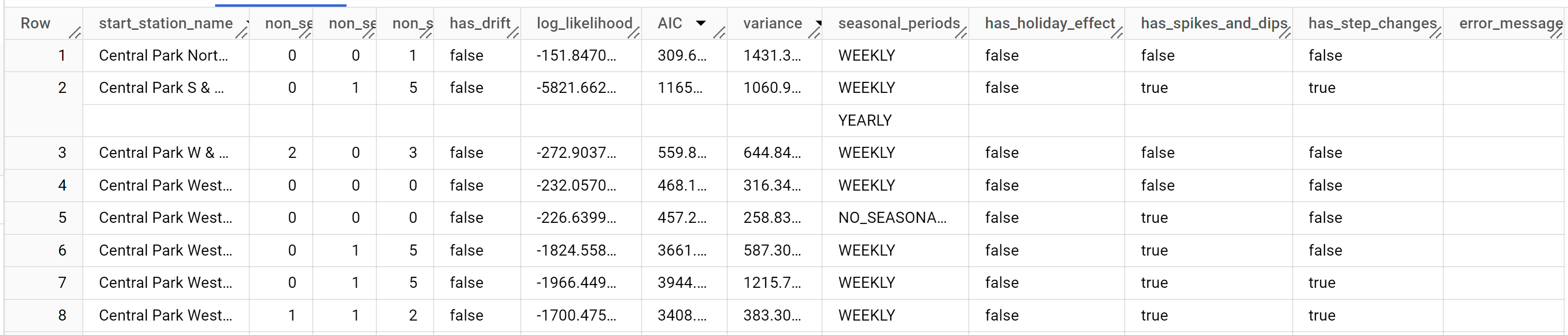
While `auto.ARIMA` evaluates dozens of candidate ARIMA models for each
time series, `ML.ARIMA_EVALUATE` by default only outputs the information of the
best model to make the output table compact. To view all the candidate models,
you can set the `ML.ARIMA_EVALUATE` function's
[`show_all_candidate_model` argument](https://docs.cloud.google.com/bigquery/docs/reference/standard-sql/bigqueryml-syntax-arima-evaluate.md.txt#arguments) to `TRUE`.
### BigQuery DataFrames
Before trying this sample, follow the BigQuery DataFrames
setup instructions in the [BigQuery quickstart
using BigQuery DataFrames](https://docs.cloud.google.com/bigquery/docs/dataframes-quickstart).
For more information, see the
[BigQuery DataFrames reference documentation](https://docs.cloud.google.com/python/docs/reference/bigframes/latest.md.txt).
To authenticate to BigQuery, set up Application Default Credentials.
For more information, see [Set
up ADC for a local development environment](https://docs.cloud.google.com/docs/authentication/set-up-adc-local-dev-environment).
```python
import bigframes.pandas as bpd
from bigframes.bigquery import ml
# Set partial ordering mode for BigQuery DataFrames.
# For more information, see the BigQuery DataFrames performance documentation:
# https://cloud.google.com/bigquery/docs/dataframes-performance#partial-ordering-mode
bpd.options.bigquery.ordering_mode = "partial"
# For more information, see the BigQuery DataFrames API reference documentation:
# https://dataframes.bigquery.dev/reference/api/bigframes.bigquery.ml.arima_evaluate.html#bigframes.bigquery.ml.arima_evaluate
ml.arima_evaluate(
your_model_id, # For example: "bqml_tutorial.nyc_citibike_arima_model",
)
# Expected output:
# start_station_name non_seasonal_p non_seasonal_d non_seasonal_q has_drift log_likelihood AIC variance ...
# 1 Central Park West & W 72 St 0 1 5 False -1966.449243 3944.898487 1215.689281 ...
# 8 Central Park W & W 96 St 0 0 5 False -274.459923 562.919847 655.776577 ...
# 9 Central Park West & W 102 St 0 0 0 False -226.639918 457.279835 258.83582 ...
# 11 Central Park West & W 76 St 1 1 2 False -1700.456924 3408.913848 383.254161 ...
# 4 Grand Army Plaza & Central Park S 0 1 5 False -5507.553498 11027.106996 624.138741 ...
```
The `start_station_name` column identifies the input data column for which
time series were created. This is the column that you specified with the
`time_series_id_col` option when creating the model.
The `non_seasonal_p`, `non_seasonal_d`, `non_seasonal_q`, and `has_drift`
output columns define an ARIMA model in the training pipeline. The
`log_likelihood`, `AIC`, and `variance` output columns are relevant to the ARIMA
model fitting process. The fitting process determines the best ARIMA model by
using the `auto.ARIMA` algorithm, one for each time series.
The `auto.ARIMA` algorithm uses the
[KPSS test](https://en.wikipedia.org/wiki/KPSS_test) to determine the best value
for `non_seasonal_d`, which in this case is `1`. When `non_seasonal_d` is `1`,
the auto.ARIMA algorithm trains 42 different candidate ARIMA models in parallel.
In this example, all 42 candidate models are valid, so the output contains 42
rows, one for each candidate ARIMA model; in cases where some of the models
aren't valid, they are excluded from the output. These candidate models are
returned in ascending order by AIC. The model in the first row has the lowest
AIC, and is considered as the best model. This best model is saved as the final
model and is used when you forecast data, evaluate the model, and
inspect the model's coefficients as shown in the following steps.
The `seasonal_periods` column contains information about the seasonal pattern
identified in the time series data. Each time series can have different seasonal
patterns. For example, from the figure, you can see that one time series has a
yearly pattern, while others don't.
The `has_holiday_effect`, `has_spikes_and_dips`, and `has_step_changes` columns
are only populated when `decompose_time_series=TRUE`. These columns also reflect
information about the input time series data, and are not related to the ARIMA
modeling. These columns also have the same values across all output rows.
## Inspect the model's coefficients
### SQL
Inspect the time series model's coefficients by using the
`ML.ARIMA_COEFFICIENTS` function.
Follow these steps to retrieve the model's coefficients:
1. In the Google Cloud console, go to the **BigQuery** page.
[Go to BigQuery](https://console.cloud.google.com/bigquery)
2. In the query editor, paste in the following query and click **Run**:
```googlesql
SELECT
*
FROM
ML.ARIMA_COEFFICIENTS(MODEL `bqml_tutorial.nyc_citibike_arima_model_group`);
```
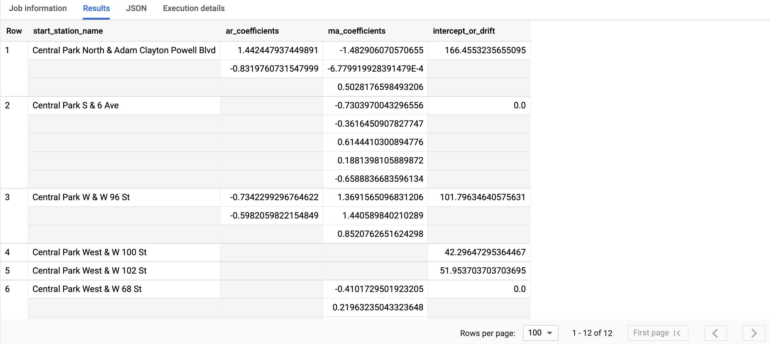
The query takes less than a second to complete. The results should look
similar to the following:
For more information about the output columns, see
[`ML.ARIMA_COEFFICIENTS` function](https://docs.cloud.google.com/bigquery/docs/reference/standard-sql/bigqueryml-syntax-arima-coefficients.md.txt).
### BigQuery DataFrames
Inspect the time series model's coefficients by using the
[`bigframes.bigquery.ml.arima_coefficients` function](https://dataframes.bigquery.dev/reference/api/bigframes.bigquery.ml.arima_coefficients.html#bigframes.bigquery.ml.arima_coefficients).
Before trying this sample, follow the BigQuery DataFrames
setup instructions in the [BigQuery quickstart
using BigQuery DataFrames](https://docs.cloud.google.com/bigquery/docs/dataframes-quickstart).
For more information, see the
[BigQuery DataFrames reference documentation](https://docs.cloud.google.com/python/docs/reference/bigframes/latest.md.txt).
To authenticate to BigQuery, set up Application Default Credentials.
For more information, see [Set
up ADC for a local development environment](https://docs.cloud.google.com/docs/authentication/set-up-adc-local-dev-environment).
```python
import bigframes.pandas as bpd
from bigframes.bigquery import ml
# Set partial ordering mode for BigQuery DataFrames.
# For more information, see the BigQuery DataFrames performance documentation:
# https://cloud.google.com/bigquery/docs/dataframes-performance#partial-ordering-mode
bpd.options.bigquery.ordering_mode = "partial"
# For more information, see the BigQuery DataFrames API reference documentation:
# https://dataframes.bigquery.dev/reference/api/bigframes.bigquery.ml.arima_coefficients.html#bigframes.bigquery.ml.arima_coefficients
ml.arima_coefficients(
your_model_id, # For example: "bqml_tutorial.nyc_citibike_arima_model",
)
# Expected output:
# start_station_name ar_coefficients ma_coefficients intercept_or_drift
# 5 Central Park West & W 68 St [] [-0.41014089 0.21979212 -0.59854213 -0.251438... 0.0
# 6 Central Park S & 6 Ave [] [-0.71488957 -0.36835772 0.61008532 0.183290... 0.0
# 0 Central Park West & W 85 St [] [-0.39270166 -0.74494638 0.76432596 0.489146... 0.0
# 3 W 82 St & Central Park West [-0.50219511 -0.64820817] [-0.20665325 0.67683137 -0.68108631] 0.0
# 11 W 106 St & Central Park West [-0.70442887 -0.66885553 -0.25030325 -0.34160669] [] 0.0
```
The `start_station_name` column identifies the input data column for which
time series were created. This is the column that you specified in the
`time_series_id_col` option when creating the model.
The `ar_coefficients` output column shows the model coefficients of the
autoregressive (AR) part of the ARIMA model. Similarly, the `ma_coefficients`
output column shows the model coefficients of the moving-average (MA) part of
the ARIMA model. Both of these columns contain array values, whose lengths are
equal to `non_seasonal_p` and `non_seasonal_q`, respectively. The
`intercept_or_drift` value is the constant term in the ARIMA model.
## Use the model to forecast data
### SQL
Forecast future time series values by using the `ML.FORECAST`
function.
In the following GoogleSQL query, the
`STRUCT(3 AS horizon, 0.9 AS confidence_level)` clause indicates that the
query forecasts 3 future time points, and generates a prediction interval
with a 90% confidence level.
Follow these steps to forecast data with the model:
1. In the Google Cloud console, go to the **BigQuery** page.
[Go to BigQuery](https://console.cloud.google.com/bigquery)
2. In the query editor, paste in the following query and click **Run**:
```googlesql
SELECT
*
FROM
ML.FORECAST(MODEL `bqml_tutorial.nyc_citibike_arima_model_group`,
STRUCT(3 AS horizon, 0.9 AS confidence_level))
```
3. Click **Run**.
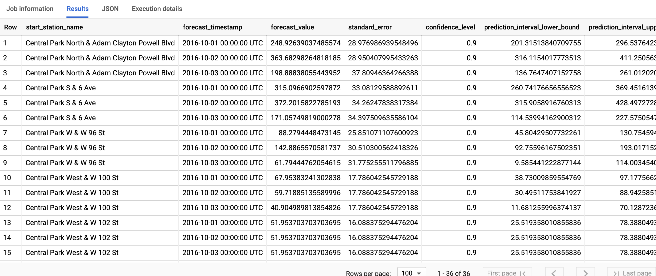
The query takes less than a second to complete. The results should look
like the following:
For more information about the output columns, see
[`ML.FORECAST` function](https://docs.cloud.google.com/bigquery/docs/reference/standard-sql/bigqueryml-syntax-forecast.md.txt).
### BigQuery DataFrames
Forecast future time series values by using the
[`bigframes.bigquery.ml.forecast` function](https://dataframes.bigquery.dev/reference/api/bigframes.bigquery.ml.forecast.html#bigframes.bigquery.ml.forecast).
Before trying this sample, follow the BigQuery DataFrames
setup instructions in the [BigQuery quickstart
using BigQuery DataFrames](https://docs.cloud.google.com/bigquery/docs/dataframes-quickstart).
For more information, see the
[BigQuery DataFrames reference documentation](https://docs.cloud.google.com/python/docs/reference/bigframes/latest.md.txt).
To authenticate to BigQuery, set up Application Default Credentials.
For more information, see [Set
up ADC for a local development environment](https://docs.cloud.google.com/docs/authentication/set-up-adc-local-dev-environment).
```python
import bigframes.pandas as bpd
from bigframes.bigquery import ml
# Set partial ordering mode for BigQuery DataFrames.
# For more information, see the BigQuery DataFrames performance documentation:
# https://cloud.google.com/bigquery/docs/dataframes-performance#partial-ordering-mode
bpd.options.bigquery.ordering_mode = "partial"
# For more information, see the BigQuery DataFrames API reference documentation:
# https://dataframes.bigquery.dev/reference/api/bigframes.bigquery.ml.forecast.html#bigframes.bigquery.ml.forecast
ml.forecast(
your_model_id, # For example: "bqml_tutorial.nyc_citibike_arima_model",
horizon=3,
confidence_level=0.9,
)
# Expected output:
# forecast_timestamp start_station_name forecast_value standard_error confidence_level ...
# 4 2016-10-01 00:00:00+00:00 Central Park S & 6 Ave 302.377201 32.572948 0.9 ...
# 14 2016-10-02 00:00:00+00:00 Central Park North & Adam Clayton Powell Blvd 263.917567 45.284082 0.9 ...
# 1 2016-09-25 00:00:00+00:00 Central Park West & W 85 St 189.574706 39.874856 0.9 ...
# 20 2016-10-02 00:00:00+00:00 Central Park West & W 72 St 175.474862 40.940794 0.9 ...
# 12 2016-10-01 00:00:00+00:00 W 106 St & Central Park West 63.88163 18.088868 0.9 ...
```
The first column, `start_station_name`, annotates the time series that each
time series model is fitted against. Each `start_station_name` has three
rows of forecasted results, as specified by the `horizon` value.
For each `start_station_name`, the output rows are in chronological order by the
`forecast_timestamp` column value. In time series forecasting, the prediction
interval, as represented by the `prediction_interval_lower_bound` and
`prediction_interval_upper_bound` column values, is as important as the
`forecast_value` column value. The `forecast_value` value is the middle point
of the prediction interval. The prediction interval depends on the
`standard_error` and `confidence_level` column values.
## Explain the forecasting results
### SQL
You can get explainability metrics in addition to forecast data by using the
`ML.EXPLAIN_FORECAST` function. The `ML.EXPLAIN_FORECAST` function forecasts
future time series values and also returns all the separate components of the
time series. If you just want to return forecast data, use the `ML.FORECAST`
function instead, as shown in
[Use the model to forecast data](https://docs.cloud.google.com/bigquery/docs/arima-multiple-time-series-forecasting-tutorial.md.txt#use_the_model_to_forecast_data).
The `STRUCT(3 AS horizon, 0.9 AS confidence_level)` clause used in the
`ML.EXPLAIN_FORECAST` function indicates that the query forecasts 3 future
time points and generates a prediction interval with 90% confidence.
Follow these steps to explain the model's results:
1. In the Google Cloud console, go to the **BigQuery** page.
[Go to BigQuery](https://console.cloud.google.com/bigquery)
2. In the query editor, paste in the following query and click **Run**:
```googlesql
SELECT
*
FROM
ML.EXPLAIN_FORECAST(MODEL `bqml_tutorial.nyc_citibike_arima_model_group`,
STRUCT(3 AS horizon, 0.9 AS confidence_level));
```
The query takes less than a second to complete. The results should look
like the following:


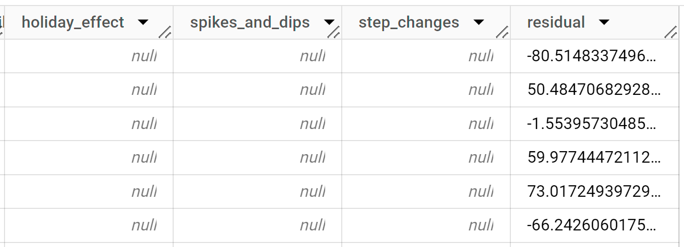
The first thousand rows returned are all history data. You must scroll
through the results to see the forecast data.
The output rows are ordered first by `start_station_name`, then
chronologically by the `time_series_timestamp` column value. In time series
forecasting, the prediction
interval, as represented by the `prediction_interval_lower_bound` and
`prediction_interval_upper_bound` column values, is as important as the
forecast value. For rows that have a value of `forecast` in the
`time_series_type` column, the `time_series_data` column contains the
forecast value. The prediction interval depends on the
`standard_error` and `confidence_level` column values.
For more information about the output columns, see
[`ML.EXPLAIN_FORECAST`](https://docs.cloud.google.com/bigquery/docs/reference/standard-sql/bigqueryml-syntax-explain-forecast.md.txt).
### BigQuery DataFrames
You can get explainability metrics in addition to forecast data by using the
[`bigframes.bigquery.ml.explain_forecast` function](https://dataframes.bigquery.dev/reference/api/bigframes.bigquery.ml.explain_forecast.html#bigframes.bigquery.ml.explain_forecast).
The `bigframes.bigquery.ml.explain_forecast` function forecasts
future time series values and also returns all the separate components of the
time series. If you just want to return forecast data, use the
`bigframes.bigquery.ml.forecast` function instead, as shown in
[Use the model to forecast data](https://docs.cloud.google.com/bigquery/docs/arima-multiple-time-series-forecasting-tutorial.md.txt#use_the_model_to_forecast_data).
The `horizon=3, confidence_level=0.9` arguments used in the
`bigframes.bigquery.ml.explain_forecast` function indicate that the query
forecasts 3 future time points and generates a prediction interval with 90%
confidence.
Before trying this sample, follow the BigQuery DataFrames
setup instructions in the [BigQuery quickstart
using BigQuery DataFrames](https://docs.cloud.google.com/bigquery/docs/dataframes-quickstart).
For more information, see the
[BigQuery DataFrames reference documentation](https://docs.cloud.google.com/python/docs/reference/bigframes/latest.md.txt).
To authenticate to BigQuery, set up Application Default Credentials.
For more information, see [Set
up ADC for a local development environment](https://docs.cloud.google.com/docs/authentication/set-up-adc-local-dev-environment).
```python
import bigframes.pandas as bpd
from bigframes.bigquery import ml
# Set partial ordering mode for BigQuery DataFrames.
# For more information, see the BigQuery DataFrames performance documentation:
# https://cloud.google.com/bigquery/docs/dataframes-performance#partial-ordering-mode
bpd.options.bigquery.ordering_mode = "partial"
# For more information, see the BigQuery DataFrames API reference documentation:
# https://dataframes.bigquery.dev/reference/api/bigframes.bigquery.ml.explain_forecast.html#bigframes.bigquery.ml.explain_forecast
ml.explain_forecast(
your_model_id, # For example: "bqml_tutorial.nyc_citibike_arima_model",
horizon=3,
confidence_level=0.9,
)
# Expected output:
# time_series_timestamp start_station_name time_series_type time_series_data time_series_adjusted_data standard_error confidence_level prediction_interval_lower_bound prediction_interval_upper_bound trend seasonal_period_yearly seasonal_period_quarterly seasonal_period_monthly seasonal_period_weekly seasonal_period_daily holiday_effect spikes_and_dips step_changes residual
# 0 2013-07-01 00:00:00+00:00 Central Park S & 6 Ave history 69.0 154.168527 32.572948 0.0 35.477484 -28.402102 0.0 -85.168527 147.093145
# 1 2013-07-01 00:00:00+00:00 Grand Army Plaza & Central Park S history 79.0 79.0 24.982769 0.0 43.46428 -30.01599 0.0 0.0 65.55171
# 2 2013-07-02 00:00:00+00:00 Central Park S & 6 Ave history 180.0 204.045651 32.572948 147.093045 72.498327 -15.545721 0.0 -85.168527 61.122876
# 3 2013-07-02 00:00:00+00:00 Grand Army Plaza & Central Park S history 129.0 99.556269 24.982769 65.551665 45.836432 -11.831828 0.0 0.0 29.443731
# 4 2013-07-03 00:00:00+00:00 Central Park S & 6 Ave history 115.0 205.968236 32.572948 191.32754 59.220766 -44.580071 0.0 -85.168527 -5.799709
```
The output contains one row per time point for each `start_station_name`.
In time series forecasting, the prediction
interval, as represented by the `prediction_interval_lower_bound` and
`prediction_interval_upper_bound` column values, is as important as the
forecast value. For rows that have a value of `forecast` in the
`time_series_type` column, the `time_series_data` column contains the
forecast value. The prediction interval depends on the
`standard_error` and `confidence_level` column values.
## Clean up
To avoid incurring charges to your Google Cloud account for the resources used in this
tutorial, either delete the project that contains the resources, or keep the project and
delete the individual resources.
- You can delete the project you created.
- Or you can keep the project and delete the dataset.
### Delete your dataset
Deleting your project removes all datasets and all tables in the project. If you
prefer to reuse the project, you can delete the dataset you created in this
tutorial:
1. If necessary, open the BigQuery page in the
Google Cloud console.
[Go to the BigQuery page](https://console.cloud.google.com/bigquery)
2. In the navigation, click the **bqml_tutorial** dataset you created.
3. Click **Delete dataset** to delete the dataset, the table, and all of the
data.
4. In the **Delete dataset** dialog, confirm the delete command by typing
the name of your dataset (`bqml_tutorial`) and then click **Delete**.
### Delete your project
To delete the project:
> [!CAUTION]
> **Caution** : Deleting a project has the following effects:
>
> - **Everything in the project is deleted.** If you used an existing project for the tasks in this document, when you delete it, you also delete any other work you've done in the project.
> - **Custom project IDs are lost.** When you created this project, you might have created a custom project ID that you want to use in the future. To preserve the URLs that use the project ID, such as an `appspot.com` URL, delete selected resources inside the project instead of deleting the whole project.
>
>
> If you plan to explore multiple architectures, tutorials, or quickstarts, reusing projects
> can help you avoid exceeding project quota limits.
1. In the Google Cloud console, go to the **Manage resources** page.
[Go to Manage resources](https://console.cloud.google.com/iam-admin/projects)
2. In the project list, select the project that you want to delete, and then click **Delete**.
3. In the dialog, type the project ID, and then click **Shut down** to delete the project.
## What's next
- Learn how to [forecast a single time series with a univariate model](https://docs.cloud.google.com/bigquery/docs/arima-single-time-series-forecasting-tutorial.md.txt)
- Learn how to [forecast a single time series with a multivariate model](https://docs.cloud.google.com/bigquery/docs/arima-plus-xreg-single-time-series-forecasting-tutorial.md.txt)
- Learn how to [scale a univariate model when forecasting multiple time series over many rows](https://docs.cloud.google.com/bigquery/docs/arima-speed-up-tutorial.md.txt).
- Learn how to [hierarchically forecast multiple time series with a univariate model](https://docs.cloud.google.com/bigquery/docs/arima-time-series-forecasting-with-hierarchical-time-series.md.txt)
- For an overview of BigQuery ML, see [Introduction to AI and ML in BigQuery](https://docs.cloud.google.com/bigquery/docs/bqml-introduction.md.txt).